CIMA - C3 Fundamentals Of Business Mathematics

Подождите немного. Документ загружается.

300 11: Forecasting ⏐ Part F Forecasting

(a) It assumes a linear relationship exists between the two variables (since linear regression analysis

produces an equation in the linear format) whereas a non-linear relationship might exist.

(b) It

assumes that the value of one variable, Y, can be predicted or estimated from the value of one

other variable, X

. In reality the value of Y might depend on several other variables, not just X.

it assumes that what has happened in the past will provide a

reliable guide to the future

(d) When calculating a line of best fit, there will be a range of values for X. In the example in Paragraph

6.2, Chapter 10, the line Y = 28 + 2.6X was predicted from data with output values ranging from X =

16 to X = 24. Depending on the degree of correlation between X and Y, we might safely use the

estimated line of best fit to predict values for Y in the future, provided that the value of X remains

within the range 16 to 24. We would be on less safe ground if we used the formula to predict a value

for Y when X = 10, or 30, or any other value outside the range 16 to 24, because we would have to

assume that the trend line applies outside the range of X values used to establish the line in the

first place

(e) As with any forecasting process,

the amount of data available is very important. Even if correlation

is high, if we have fewer than about ten pairs of values, we must regard any forecast as being

somewhat unreliable. (It is likely to provide more reliable forecasts than the scattergraph method,

however, since it uses all of the available data.)

(f)

The reliability of a forecast will depend on the reliability of the data collected to determine the

regression analysis equation

. If the data is not collected accurately or if data used is false, forecasts

are unlikely to be acceptable.

Chapter Roundup

• A time series is a series of figures or values recorded over time. Any pattern found in the data is then assumed to

continue into the future and an extrapolative forecast is produced.

• There are four components of a time series: trend, seasonal variations, cyclical variations and random

variations.

• The trend is the underlying long-term movement over time in the values of the data recorded.

• Seasonal variations are short-term fluctuations in recorded values, due to different circumstances which affect

results at different times of the year, on different days of the week or at different times of the day etc.

• Cyclical variations are medium-term changes in results caused by circumstances which repeat in cycles.

• One method of finding the trend is by the use of moving averages.

• When finding the moving average of an even number of results, a second moving average has to be calculated so

that trend values can relate to specific actual figures.

• Seasonal variations are the difference between actual and trend figures. An average of the seasonal variations

for each time period within the cycle must be determined and then adjusted so that the total of the seasonal

variations sums to zero. Seasonal variations can be estimated using the additive model (Y = T + S + R, with

seasonal variations = Y – T) or the multiplicative model (Y = T × S × R, with seasonal variations = Y/T).

• Forecasts can be made by extrapolating the trend and adjusting for seasonal variations.

• There are a number of factors which will affect the reliability of forecasts. Remember that all forecasts are subject

to error.

Part F Forecasting ⏐ 11: Forecasting 301

Quick Quiz

1 If the trend is increasing or decreasing over time, it is better to use the additive model for forecasting.

True

False

Results Method

Odd number of time periods Calculate 1 moving average

Even number of time periods Calculate 2 moving averages

3 When deseasonalising data, the following rules apply to the additive model.

I Add positive seasonal variations

II Subtract positive seasonal variations

III Add negative seasonal variations

IV Subtract negative seasonal variations

A I and II

B II and III

C II and IV

D I only

4 Cyclical variation is the term used for the difference which is not explained by the trend line and the average

seasonal variation.

True

False

5 The trend for profit (y) is related to time (t) by the equation y = 50 + 1.5t.

What is the estimate of the profit to the nearest $ at time t = 21 if the seasonal component at that point is 0.9 using

a multiplicative model?

6 Unemployment last quarter was 738,000. The trend figure for that quarter was 700,000 and the seasonal factor

using the additive model was – 17,500.

What is the seasonally adjusted unemployment figure for the last quarter?

]

[

302 11: Forecasting ⏐ Part F Forecasting

Answers to Quick Quiz

1 False

2 Odd number of time periods = calculate 1 moving average

Even number of time periods = calculate 2 moving averages

3 B

4 False. The residual is the term used to explain the difference which is not explained by the trend line and the

average seasonal variation.

5 y = 50 + (1.5 × 21)

= 81.5

Forecast = 81.5 × 0.9

= 73.35

6 The seasonally adjusted value is an estimate of the trend.

Trend = Actual value – Seasonal component

= 738,000 – (–17,500)

= 755,500

Now try the questions below from the Exam Question Bank

Question numbers Pages

89-99 348-354

755,500

303

Part G

Spreadsheets

304

305

Topic list Syllabus references

1 Uses of spreadsheet software G, (i),(ii),(1),(3)

2 Spreadsheet design G, (i),(ii),(iii),(1)

3 Advantages and disadvantages of

spreadsheets

G, (ii),(2)

Spreadsheets

Introduction

Spreadsheet skills are essential for people working in a management accounting environment

as much of the information produced is analysed or presented using spreadsheet software.

We have already looked at some of the features and functions of Excel in earlier chapters.

This chapter will summarise the functions which you need to be familiar with and also look at

the advantages and disadvantages of spreadsheets.

306 12: Spreadsheets ⏐ Part G Spreadsheets

1 Uses of spreadsheet software

Spreadsheets can be used in a variety of accounting contexts. You should practise using spreadsheets, hands-on

experience is the key to spreadsheet proficiency.

1.1 Uses of spreadsheets by Chartered Management Accountants

Some common applications of spreadsheets are:

• Preparation of management accounts

• Cash flow analysis, budgeting and forecasting

• Account reconciliation

• Revenue and cost analysis

• Comparison and variance analysis

• Sorting, filtering and categorising large volumes of data

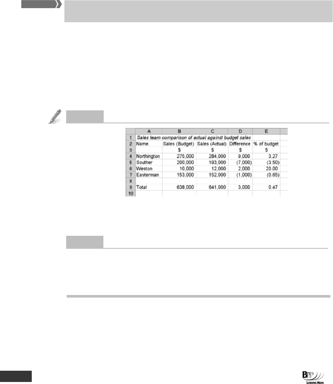
Question

Actual sales compared with budget sales

Give a suitable formula for each of the following cells.

(a) Cell D4

(b) Cell E6

Answe

(a) =C4-B4.

(b) =(D6/B6)*100.

percentages are based on different quantities.

T F

RWAR

Part G Spreadsheets ⏐ 12: Spreadsheets 307

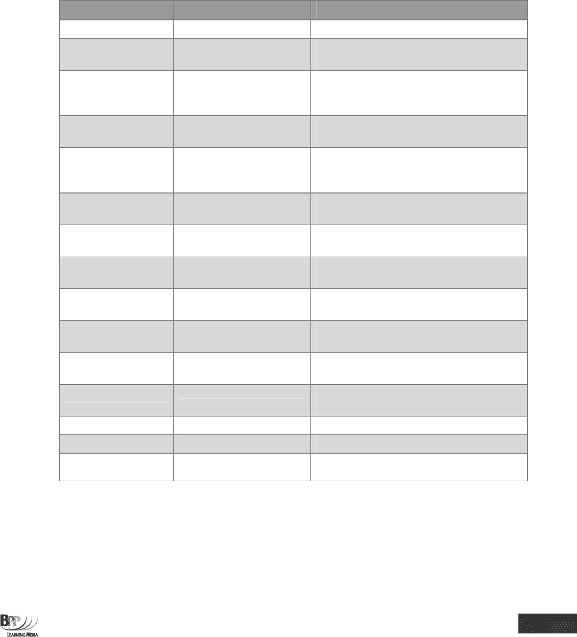
1.2 Summary of Excel functions

Throughout this Study Text, we have looked at the specific use of Excel to perform tasks. Here is a summary of the

functions that have been covered and that you will need to be able to use in your assessment.

Excel function Example What it does

SUM =SUM(C1:C5) Adds the values in the selected range of cells

ROUND =ROUND(A3*3,2) Rounds the result of the calculation to a specified

number of decimal places

COUNT =COUNT(C1:C5) This will return the number of entries (actually

counts each cell that contains number data) in the

selected range of cells

NOW =NOW() The time and date as set on the computer will be

inserted into the cell

IF =IF(C2>1,"Yes","No") The IF function will check the logical condition of a

statement and return one value if true and a

different value if false

FREQUENCY =FREQUENCY(A3:D7,F3:F9) Calculates the frequency ie how often values occur

within a range of values

AVERAGE =AVERAGE(C1:C5) Finds the mean of the values in the selected range

of cells. Used to calculate ROI.

MAX =MAX(C1:C5) This will return the largest (max) value in the

selected range of cells

MIN

=MIN(C1:C5)

This will return the smallest (Min) value in the

selected range of cells

MEDIAN

=MEDIAN(C1:C5)

This will return the median value in the selected

range of cells

MODE

=MODE(C1:C5)

This will return the value of the mode in a selected

range of cells

STDEV

=STDEV(C1:C5)

This will return the standard deviation of a range of

data

NPV

=NPV(B10,B4:B7)-B3

Used to calculate the net present value

IRR

=IRR(B3:B7,0.05)

Used to calculate the internal rate of return

FORECAST

=FORECAST(B3,$C$3:$C$7,$B

$3:$B$7)

Used to plot a regression line

308 12: Spreadsheets ⏐ Part G Spreadsheets

2 Spreadsheet design

The design, structure and presentation of a spreadsheet are essential aspects which contribute to its effectiveness.

2.1 Characteristics of a useful spreadsheet

A good spreadsheet will have the following attributes.

(a) It is as error free as possible.

(b) It is simple to use and can be used with minimal training and control procedures.

(d) It can be changed easily.

(e) It will produce the required results.

In order to achieve these characteristics, the following rules should be followed.

(a) Split the spreadsheet into three sections: input data, calculations, results.

(b) Use titles to define the purpose of the spreadsheet.

(d) Include author details so that it is clear who is responsible for the accuracy and maintenance of the

spreadsheet.

(e) Define the source of the data used and include the data or range of data used in the calculations.

(f) Date the spreadsheet so that it is clear which version is being used and when it was updated. The

NOW() function is useful here (see paragraph 1.2).

(g) Use consistent cell formatting and rounding. The ROUND function will ensure that the results of a

calculation are rounded to a specific number of decimal places (see Chapter 1, paragraph 7.4.2).

(h) Use colours, borders and shading to differentiate and highlight key data.

(i) Include supporting documentation and information. This can be achieved with the INSERT

COMMENT command. A small red triangle on the cell will indicate where a comment has been

inserted.

(j) Include control checks using the IF function or cross-checks on calculations.

2.2 Other aspects

2.2.1 Three dimensional (multi-sheet) spreadsheets

Spreadsheet packages permit the user to work with multiple sheets that refer to each other. For example, suppose

you were producing a profit forecast for two regions, and a combined forecast for the total of the regions. This

situation would be suited to using separate worksheets for each region and another for the total. This approach is

sometimes referred to as working in three dimensions, as you are able to flip between different sheets stacked in

front or behind each other. Cells in one sheet may refer to cells in another sheet. So, in our example, the formulae

in the cells in the total sheet would refer to the cells in the other sheets.

Excel has a series of 'tabs', one for each worksheet at the foot of the spreadsheet.

T F

RWAR

Part G Spreadsheets ⏐ 12: Spreadsheets 309

There are a wide range of situations suited to the multi-sheet approach.

(a) A model could use one sheet for variables, a second for calculations, and a third for outputs.

(b) To enable quick and easy consolidation of similar sets of data, for example the financial results of

two subsidiaries or the budgets of two departments.

product code order and another sorted in product name order.

2.2.2 Macros

A macro is an automated process that may be written by recording key-strokes and mouse clicks. A macro is a

sort of mini-program that automates keystrokes or actions. Macros are often used within spreadsheets. Macros

may be written using a type of code – like a programming language. However, most spreadsheet users produce

macros by asking the spreadsheet to record their actions – this automatically generates the macro 'code' required.

2.2.3 Templates

A template is a spreadsheet which contains the formulae required, but the data has been removed. The

spreadsheet is saved as a template and different data can then be entered as necessary. The spreadsheet is

protected so the user can only input data into the input cells.

2.2.4 Data input forms

A further development of a template is to remove the data from the main worksheet and put it on data input forms

on separate worksheets. This enables the data to be input and checked more easily.

3 Advantages and disadvantages of spreadsheets

3.1 Advantages of spreadsheets

• Excel is easy to learn and to use

• Spreadsheets make the calculation and manipulation of data easier and quicker

• They enable the analysis, reporting and sharing of financial information

• They enable 'what-if' analysis to be performed very quickly

3.2 Disadvantages of spreadsheets

• A spreadsheet is only as good as its original design, garbage in = garbage out!

• Formulae are hidden from sight so the underlying logic of a set of calculations may not be obvious

• A spreadsheet presentation may make reports appear infallible

• Research shows that a high proportion of large models contain critical errors

• A database may be more suitable to use with large volumes of data

• Spreadsheets can easily be corrupted and it is difficult to find errors in large models