Brizard A. An Introduction to Lagrangian Mechanics

Подождите немного. Документ загружается.

2.2. PRINCIPLE OF LEAST ACTION OF EULER AND LAGRANGE 25

with ∇F =

r −tan α

z. The surface co ordinates can be chosen to be the polar angle θ and

the function

s(x, y, z)=

+ y

+ z

which measures the distance from the apex of the cone (deﬁning the origin), so that

∂x

∂θ

= r

θ = r

z ×

r and

∂x

∂s

= sin α

r + cos α

z =

with

∂x

∂θ

∂x

∂s

= r cos α ∇F

and J = r cos α. Lastly, the velocity of the particle is

x =˙s

s + r

θ and, thus, it satisﬁes

x · ∇F = 0. We shall return to this example in Sec. 2.4.4.

2.2.3 Euler-Lagrange Equations

The Principle of Least Action (also known as Hamilton’s principle as it is formulated here)

is expressed in terms of a function L(q,

q; t) known as the Lagrangian, which appears in

the action integral

S[q]=

L(q,

q; t) dt, (2.8)

where the action integral is a functional of the vector function q(t), which provides a path

from the initial point q

= q(t

) to the ﬁnal point q

= q(t

). The variational principle

0=δS[q]=

d

S[q + δq]

=0

δq ·

∂L

∂q

−

∂L

∂

dt,

where the variation δq is assumed to vanish at the integration boundaries (δq

=0=δq

yields the Euler-Lagrange equation for the generalized coordinate q

(j =1, ..., k)

∂L

∂ ˙q

∂L

∂q

. (2.9)

The Lagrangian also satisﬁes the second Euler equation

L −

∂L

∂

∂L

∂t

, (2.10)

and thus, for time-independent Lagrangian systems (∂L/∂t = 0), we ﬁnd that L−

q ∂L/∂

is a conserved quantity whose interpretation will b e discussed shortly.

The form of the Lagrangian function L( r,

r; t) is dictated by our requirement that

Newton’s Second Law m

r = −∇U(r,t), which describes the motion of a particle of mass

26 CHAPTER 2. LAGRANGIAN MECHANICS

m in a nonuniform (possibly time-dependent) potential U(r,t), be written in the Euler-

Lagrange form (2.9). One easily obtains the form

L(r,

r; t)=

− U(r,t), (2.11)

for the Lagrangian of a particle of mass m, which is simply the kinetic energy of the

particle minus its potential energy. The minus sign in Eq. (2.11) is important; not only

does this form give us the correct equations of motion but, without the minus sign, energy

would not be conserved. In fact, we note that Jacobi’s action integral (2.7) can also be

written as A =

[(K − U)+E] dt, using the Energy conservation law E = K + U; hence,

Energy conservation is the important connection between the Principles of Least Action of

Maupertuis-Jacobi and Euler-Lagrange.

For a simple mechanical system, the Lagrangian function is obtained by computing the

kinetic energy of the system and its potential energy and then construct Eq. (2.11). The

construction of a Lagrangian function for a system of N particles proceeds in three steps

as follows.

• Step I. Deﬁne k generalized coordinates {q

(t), ..., q

(t)} that represent the instanta-

neous conﬁguration of the mechanical system of N particles at time t.

• Step II. For each particle, construct the position vector r

(q; t) in Cartesian coordinates

and its associated velocity

(q,

q; t)=

∂r

∂t

j=1

˙q

∂r

∂q

for a =1, ..., N.

• Step III. Construct the kinetic energy

K(q ,

q; t)=

(q,

q; t)|

and the potential energy

U(q; t)=

U(r

(q; t),t)

for the system and combine them to obtain the Lagrangian

L(q,

q; t)=K(q,

q; t) − U(q; t).

From this Lagrangian L(q,

q; t), the Euler-Lagrange equations (2.9) are derived for each

generalized coordinate q

∂r

∂q

· m

∂v

∂q

−

∂r

∂q

· ∇U

, (2.12)

where we have used the identity ∂v

/∂ ˙q

= ∂r

/∂q

2.3. LAGRANGIAN MECHANICS IN CONFIGURATION SPACE 27

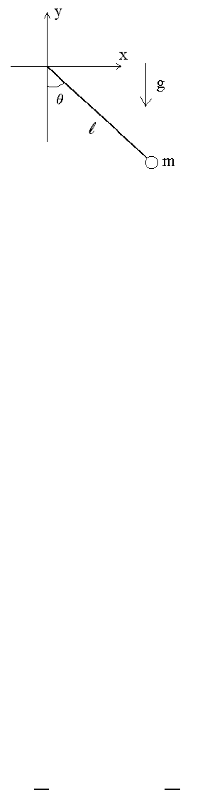
Figure 2.3: Generalized coordinates for the pendulum problem

2.3 Lagrangian Mechanics in Conﬁguration Space

In this Section, we explore the Lagrangian formulation of several mechanical systems listed

here in order of increasing complexity. As we proceed with our examples, we should realize

how the Lagrangian formulation maintains its relative simplicity compared to the applica-

tion of the more familiar Newton’s method (Isaac Newton, 1643-1727) associated with the

composition of forces.

2.3.1 Example I: Pendulum

As a ﬁrst example, we consider a pendulum composed of an object of mass m and a massless

string of constant length ` in a constant gravitational ﬁeld with acceleration g. Although

the motion of the pendulum is two-dimensional, a single generalized coordinate is needed

to describe the conﬁguration of the pendulum: the angle θ measured from the negative

y-axis (see Figure 2.3). Here, the position of the object is given as

x(θ)=` sin θ and y(θ)=−` cos θ,

with associated velocity components

˙x(θ,

θ)=`

θ cos θ and ˙y(θ,

θ)=`

θ sin θ.

Hence, the kinetic energy of the pendulum is

K =



˙x

+˙y



and choosing the zero potential energy p oint when θ = 0 (see Figure above), the gravita-

tional potential energy is

U = mg` (1 − cos θ).

28 CHAPTER 2. LAGRANGIAN MECHANICS

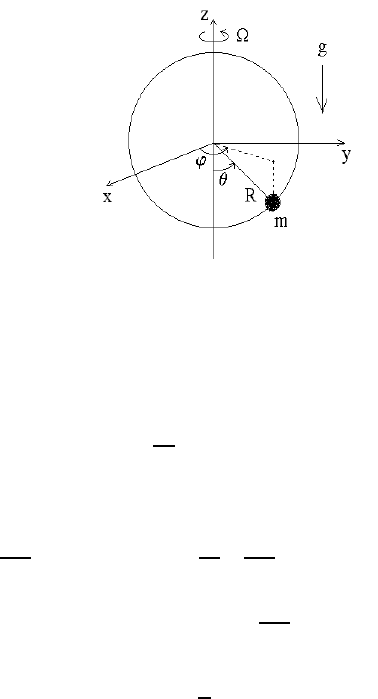
Figure 2.4: Generalized coordinates for the bead-on-a-rotating-hoop problem

The Lagrangian L = K − U is, therefore, written as

L(θ,

θ)=

− mg` (1 − cos θ),

and the Euler-Lagrange equation for θ is

∂L

∂

= m`

θ →

∂L

∂

= m`

∂L

∂θ

= −mg` sin θ

θ +

sin θ =0

The pendulum problem is solved in the next Chapter through the use of the Energy method

(a simpliﬁed version of the Hamiltonian method). Note that, whereas the tension in the

pendulum string must be considered explicitly in the Newtonian method, the string tension

is replaced by the constraint ` = constant in the Lagrangian method.

2.3.2 Example II: Bead on a Rotating Hoop

As a second example, we consider a bead of mass m sliding freely on a hoop of radius R

rotating with angular velocity Ω in a constant gravitational ﬁeld with acceleration g. Here,

since the bead of the rotating ho op moves on the surface of a sphere of radius R, we use

the generalized coordinates given by the two angles θ (measured from the negative z-axis)

and ϕ (measured from the positive x-axis), where ˙ϕ = Ω. The position of the bead is given

x(θ, t)=R sin θ cos(ϕ

+Ωt),

y(θ, t)=R sin θ sin(ϕ

+Ωt),

z(θ, t)=− R cos θ,

2.3. LAGRANGIAN MECHANICS IN CONFIGURATION SPACE 29

where ϕ( t)=ϕ

+Ωt, and its associated velocity components are

˙x(θ,

θ; t)=R



θ cos θ cos ϕ − Ω sin θ sin ϕ



˙y(θ,

θ; t)=R



θ cos θ sin ϕ + Ω sin θ cos ϕ



˙z(θ,

θ; t)=R

θ sin θ,

so that the kinetic energy of the bead is

K(θ,

θ)=

|v|



+Ω

sin



The gravitational potential energy is

U(θ)=mgR (1 − cos θ),

where we chose the zero potential energy point at θ = 0 (see Figure 2.4). The Lagrangian

L = K −U is, therefore, written as

L(θ,

θ)=



+Ω

sin



− mgR (1 −cos θ),

and the Euler-Lagrange equation for θ is

∂L

∂

= mR

θ →

∂L

∂

= mR

∂L

∂θ

= −mgR sin θ

+ mR

Ω

cos θ sin θ

θ + sin θ



− Ω

cos θ



Note that the support force provided by the hoop (necessary in the Newtonian method)

is now replaced by the constraint R = constant in the Lagrangian method. Furthermore,

although the motion intrinsically takes place on the surface of a sphere of radius R, the

azimuthal motion is completely determined by the equation ϕ(t)=ϕ

+Ωt and, thus, the

motion of the bead takes place in one dimension.

Lastly, we note that this equation displays bifurcation behavior which is investigated in

Chapter 8. For Ω

<g/R, the equilibrium point θ = 0 is stable while, for Ω

>g/R, the

equilibrium point θ = 0 is now unstable and the new equilibrium point θ = arccos(g/Ω

is stable.

30 CHAPTER 2. LAGRANGIAN MECHANICS

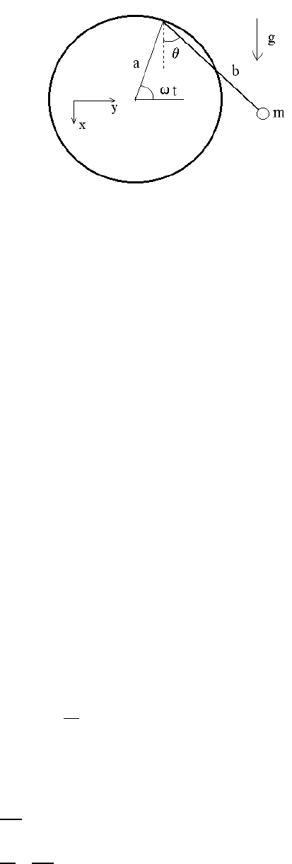
Figure 2.5: Generalized coordinates for the rotating-pendulum problem

2.3.3 Example III: Rotating Pendulum

As a third example, we consider a pendulum of mass m and length b attached to the edge

of a disk of radius a rotating at angular velocity ω in a constant gravitational ﬁeld with

acceleration g. Placing the origin at the center of the disk, the coordinates of the pendulum

mass are

x = −a sin ωt + b cos θ

y = a cos ωt + b sin θ

so that the velocity components are

˙x = −aω cos ωt − b

θ sin θ

˙y = −aω sin ωt + b

θ cos θ

and the squared velocity is

= a

+ b

+2ab ω

θ sin(θ − ωt).

Setting the zero potential energy at x = 0, the gravitational potential energy is

U = −mg x = mga sin ωt − mgb cos θ.

The Lagrangian L = K − U is, therefore, written as

L(θ,

θ; t)=

+ b

+2ab ω

θ sin(θ − ωt)

− mga sin ωt + mgb cos θ, (2.13)

and the Euler-Lagrange equation for θ is

∂L

∂

= mb

θ + mabω sin(θ − ωt) →

∂L

∂

= mb

θ + mabω(

θ − ω) cos(θ − ωt)

2.3. LAGRANGIAN MECHANICS IN CONFIGURATION SPACE 31

and

∂L

∂θ

= mabω

θ cos(θ − ωt) − mg b sin θ

θ +

sin θ −

cos(θ − ωt)=0

We recover the standard equation of motion for the pendulum when a or ω vanish.

Note that the terms

− mga sin ωt

in the Lagrangian (2.13) play no role in determining the dynamics of the system. In fact,

as can easily be shown, a Lagrangian L is always deﬁned up to an exact time derivative,

i.e., the Lagrangians L and L

= L − df/dt, where f(q,t) is an arbitrary function, lead to

the same Euler-Lagrange equations (see Section 2.4). In the present case,

f(t)=[(m/2) a

] t +(mga/ω) cos ωt

and thus this term can be omitted from the Lagrangian (2.13) without changing the equa-

tions of motion.

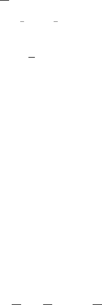
2.3.4 Example IV: Compound Atwood Machine

As a fourth (and penultimate) example, we consider a compound Atwood machine com-

posed three masses (labeled m

, m

, and m

) attached by two massless ropes through two

massless pulleys in a constant gravitational ﬁeld with acceleration g.

The two generalized coordinates for this system (see Figure 2.6) are the distance x of

mass m

from the top of the ﬁrst pulley and the distance y of mass m

from the top of the

second pulley; here, the lengths `

and `

are constants. The coordinates and velocities of

the three masses m

, m

, and m

are

= x → v

=˙x,

= `

− x + y → v

=˙y − ˙x,

= `

− x + `

− y → v

= − ˙x − ˙y,

resp ectively, so that the total kinetic energy is

K =

˙x

(˙y − ˙x)

(˙x +˙y)

Placing the zero potential energy at the top of the ﬁrst pulley, the total gravitational

potential energy, on the other hand, can be written as

U = − gx (m

− m

) − gy (m

− m

) ,

32 CHAPTER 2. LAGRANGIAN MECHANICS

Figure 2.6: Generalized coordinates for the compound-Atwo od problem

where constant terms were omitted. The Lagrangian L = K − U is, therefore, written as

L(x, ˙x, y, ˙y)=

˙x

(˙x − ˙y)

(˙x +˙y)

+ gx (m

− m

−m

)+gy (m

− m

) .

The Euler-Lagrange equation for x is

∂L

∂ ˙x

=(m

+ m

)˙x +(m

−m

)˙y →

∂L

∂ ˙x

=(m

+ m

)¨x +(m

−m

)¨y

∂L

∂x

= g (m

− m

)

while the Euler-Lagrange equation for y is

∂L

∂ ˙y

=(m

− m

)˙x +(m

+ m

)˙y →

∂L

∂ ˙y

=(m

−m

)¨x +(m

+ m

)¨y

∂L

∂y

= g (m

− m

) .

We combine these two Euler-Lagrange equations

+ m

)¨x +(m

− m

)¨y = g (m

− m

) , (2.14)

− m

)¨x +(m

+ m

)¨y = g (m

− m

) , (2.15)

2.3. LAGRANGIAN MECHANICS IN CONFIGURATION SPACE 33

to describe the dynamical evolution of the Compound Atwood Machine. This set of equa-

tions can, in fact, b e solved explicitly as

¨x = g

− ( m

− m

−

)

+(m

− m

−

)

and ¨y = g

2 m

−

+(m

− m

−

)

where m

= m

± m

. Note also that it can be shown that the position z of the center of

mass of the mechanical system (as measured from the top of the ﬁrst pulley) satisﬁes the

relation

Mg(z − z

˙x

(˙y − ˙x)

(˙x +˙y)

, (2.16)

where M =(m

+ m

) denotes the total mass of the system and we have assumed

that the system starts from rest (with its center of mass located at z

). This important

relation tells us that, as the masses start to move, the center of mass must fall.

At this point, we introduce a convenient technique (henceforth known as Freezing De-

grees of Freedom) for checking on the physical accuracy of any set of coupled Euler-Lagrange

equations. Hence, for the Euler-Lagrange equation (2.14), we may freeze the degree of free-

dom associated with the y-coordinate (i.e., we set ˙y =0=¨y or m

−

= 0) to obtain

¨x = g

− m

+ m

in agreement with the analysis of a simple Atwood machine composed of a mass m

one side and a mass m

= m

+ m

on the other side. Likewise, for the Euler-Lagrange

equation (2.15), we may freeze the degree of freedom associated with the x-coordinate (i.e.,

we set ˙x =0=¨x or m

= m

− m

−

) to obtain ¨y = g (m

−

), again in agreement

with the analysis of a simple Atwood machine.

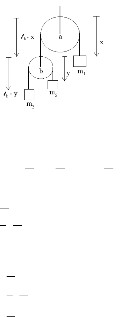
2.3.5 Example V: Pendulum with Oscillating Fulcrum

As a ﬁfth and ﬁnal example, we consider the case of a pendulum of mass m and length

` attached to a massless block which is attached to a ﬁxed wall by a massless spring of

constant k; of course, we assume that the massless block moves without friction on a set of

rails. Here, we use the two generalized coordinates x and θ shown in Figure 2.7 and write

the Cartesian co ordinates (y,z) of the pendulum mass as y = x + ` sin θ and z = −` cos θ,

with its associated velocity components v

=˙x + `

θ cos θ and v

= `

θ sin θ. The kinetic

energy of the pendulum is thus

K =



+ v





˙x

+ `

+2` cos θ ˙x



The potential energy U = U

+ U

has two terms: one term U

asso ciated with

displacement of the spring away from its equilibrium position and one term U

= mgz

asso ciated with gravity. Hence, the Lagrangian for this system is

L(x, θ, ˙x,

θ)=



˙x

+ `

+2` cos θ ˙x



−

+ mg` cos θ.

34 CHAPTER 2. LAGRANGIAN MECHANICS

Figure 2.7: Generalized coordinates for the oscillating-pendulum problem

The Euler-Lagrange equation for x is

∂L

∂ ˙x

= m



˙x + ` cos θ



→

∂L

∂ ˙x

= m ¨x + m`



θ cos θ −

sin θ



∂L

∂x

= − kx

while the Euler-Lagrange equation for θ is

∂L

∂

= m`



θ +˙x cos θ



→

∂L

∂

= m`

θ + m`



¨x cos θ − ˙x

θ sin θ



∂L

∂θ

= − m` ˙x

θ sin θ − mg` sin θ

m ¨x + kx = m`



sin θ −

θ cos θ



, (2.17)

θ +(g/`) sin θ = − (¨x/`) cos θ. (2.18)

Here, we recover the dynamical equation for a block-and-spring harmonic oscillator from

Eq. (2.17) by freezing the degree of freedom associated with the θ-coordinate (i.e., by setting