Brizard A. An Introduction to Lagrangian Mechanics
Подождите немного. Документ загружается.


3.5. ONE-DEGREE-OF-FREEDOM HAMILTONIAN DYNAMICS 55
Figure 3.2: Phase space of the pendulum
and ϕ = ±π/2 when θ = ±θ
0
, the libration solution of the pendulum problem is thus
ω
0
t(θ; E)=
Z
π/2
Θ(θ;E)
dϕ
q
1 − k
2
sin
2
ϕ
, (3.25)
where Θ(θ; E) = arcsin(k
−1
sin θ/2). The inversion of this relation yields θ(t; E) expressed
in terms of elliptic functions, while the period of oscillation is defined as
ω
0
T (E)=4
Z
π/2
0
dϕ
q
1 − k
2
sin
2
ϕ
=4
Z
π/2
0
dϕ
1+
k
2
2
sin
2
ϕ + ···
!
,
=2π
1+
k
2
4
+ ···
!
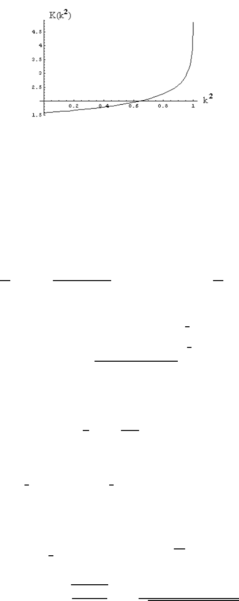
=4K(k
2
), (3.26)
where K(k
2
) denotes the complete elliptic integral of the first kind (see Figure 3.3). We
note here that if k 1 (or θ
0
1 rad) the libration perio d of a pendulum is nearly
independent of energy, T ' 2π/ω
0
. However, we also note that as E → 2 mg` (k → 1
or θ
0
→ π rad), the libration period of the pendulum becomes infinitely large (see Figure
above), i.e., T →∞as k → 1.
In this separatrix limit (θ
0
→ π), the pendulum equation (3.24) yields the separatrix
equation ˙ϕ = ω
0
cos ϕ, where ϕ = θ/2. The separatrix solution is expressed in terms of
the transcendental equation
sec ϕ(t) = cosh(ω
0
t + γ),
where cosh γ = sec ϕ
0
represents the initial condition. We again note that ϕ → π/2 (or
θ → π) only as t →∞. Separatrices are quite common in perio dic dynamical systems as
will be shown in Sec. 3.6 and Sec. 7.2.3.
56 CHAPTER 3. HAMILTONIAN MECHANICS
Figure 3.3: Pendulum period as a function of energy
3.5.3 Constrained Motion on the Surface of a Cone
The constrained motion of a particle of mass m on a cone in the presence of gravity was
shown in Sec. 2.4.4 to be doubly p eriodic in the generalized coordinates s and θ. The fact
that the Lagrangian (2.20) is independent of time leads to the conservation law of energy
E =
m
2
˙s
2
+
`
2
2m sin
2
αs
2
+ mg cos αs
!
=
m
2
˙s
2
+ V (s), (3.27)
where we have taken into account the conservation law of angular momentum ` = ms
2
sin
2
α
˙
θ.
The effective potential V (s) has a single minimum V
0
=
3
2
mgs
0
cos α at
s
0
=
`
2
m
2
g sin
2
α cos α
!
1
3
,
and the only type of motion is bounded when E>V
0
. The turning points for this problem
are solutions of the cubic equation
3
2
=
1
2σ
2
+ σ,
where = E/V
0
and σ = s/s
0
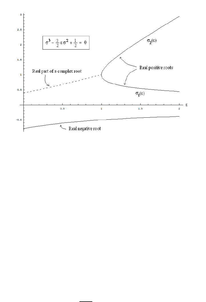
. Figure 3.4 shows the evolution of the three roots of this
equation as the normalized energy parameter is varied. The three roots ( σ
0
,σ
1
,σ
2
) satisfy
the relations σ
0
σ
1
σ
2
= −
1
2
, σ
0
+σ
1
+σ
2
=
3
2
, and σ
−1
1
+σ
−1
2
= −σ
−1
0
. We see that one root
(labeled σ
0
) remains negative for all normalized energies ; this root is unphysical since s
must be positive (by definition). On the other hand, the other two roots (σ
1
,σ
2
), which are
complex for <1 (i.e., for energies below the minumum of the effective potential energy
V
0
), become real at = 1, where σ
1
= σ
2
, and separate (σ
1
<σ
2
) for larger values of (in
the limit 1, we find σ
2
'
3
2
and σ
−1
1
'−σ
−1
0
'
√
3). Lastly, the period of oscillation
is determined by the definite integral
T ()=2
s
s
0
g cos α
Z
σ
2
σ
1
σdσ
√
3σ
2
− 1 − 2 σ
3
,
3.6. CHARGED SPHERICAL PENDULUM IN A MAGNETIC FIELD* 57
Figure 3.4: Ro ots of a cubic equation
whose solution is expressed in terms of elliptic integrals.
3.6 Charged Spherical Pendulum in a Magnetic Field*
A spherical pendulum of length ` and mass m carries a positive charge e and moves under
the action of a constant gravitational field (with acceleration g) and a constant magnetic
field B (see Figure 3.5). The position vector of the pendulum is
x = ` [ sin θ (cos ϕ
b
x + sin ϕ
b
y) − cos θ
b
z ] ,
and thus its velocity v =
˙
x is
v = `
˙
θ [ cos θ (cos ϕ
b
x + sin ϕ
b
y)+sinθ
b
z ]+` sin θ ˙ϕ (− sin ϕ
b
x + cos ϕ
b
y) ,
and the kinetic energy of the pendulum is
K =
m`
2
2
˙
θ
2
+ sin
2
θ ˙ϕ
2
.
3.6.1 Lagrangian
Because the charged pendulum moves in a magnetic field B = −B
b
z, we must include the
magnetic term v · eA/c in the Lagrangian [see Eq. (3.11)]. Here, the vector potential A

58 CHAPTER 3. HAMILTONIAN MECHANICS
Figure 3.5: Charged pendulum in a magnetic field
must b e evaluated at the p osition of the pendulum and is thus expressed as
A = −
B`
2
sin θ ( − sin ϕ
b
x + cos ϕ
b
y) ,
and, hence, we find
e
c
A · v = −
B`
2
2
sin
2
θ ˙ϕ.
Lastly, the charged pendulum is under the influence of two potential energy terms: gravi-
tational potential energy mg` (1 − cos θ) and magnetic potential energy (−µ · B = µ
z
B),
where
µ =
e
2mc
(x × v)
denotes the magnetic moment of a charge e moving about a magnetic field line. Here, it is
easy to find
µ
z
B = −
eB
2c
`
2
sin
2
θ ˙ϕ
and by combining the various terms, the Lagrangian for the system is
L(θ,
˙
θ, ˙ϕ)=m`
2
"
˙
θ
2
2
+ sin
2
θ
˙ϕ
2
2
− ω
c
˙ϕ
!#
− mg` (1 − cos θ), (3.28)
where the cyclotron frequency ω
c
is defined as ω
c
= eB/mc.

3.6. CHARGED SPHERICAL PENDULUM IN A MAGNETIC FIELD* 59
3.6.2 Euler-Lagrange equations
The Euler-Lagrange equation for θ is
∂L
∂
˙
θ
= m`
2
˙
θ →
d
dt
∂L
∂
˙
θ
!
= m`
2
¨
θ
∂L
∂θ
= −mg` sin θ + m`
2
˙ϕ
2
− 2 ω
c
˙ϕ
sin θ cos θ
or
¨
θ +
g
`
sin θ =
˙ϕ
2
− 2 ω
c
˙ϕ
sin θ cos θ
The Euler-Lagrange equation for ϕ immediately leads to a constant of the motion for the
system since the Lagrangian (3.28) is independent of the azimuthal angle ϕ and hence
p
ϕ
=
∂L
∂ ˙ϕ
= m`
2
sin
2
θ (˙ϕ − ω
c
)
is a constant of the motion, i.e., the Euler-Lagrange equation for ϕ states that ˙p
ϕ
=0.
Since p
ϕ
is a constant of the motion, we can use it the rewrite ˙ϕ in the Euler-Lagrange
equation for θ as
˙ϕ = ω
c
+
p
ϕ
m`
2
sin
2
θ
,
and thus
˙ϕ
2
− 2 ω
c
˙ϕ =
p
ϕ
m`
2
sin
2
θ
2
− ω
2
c
so that
¨
θ +
g
`
sin θ = sin θ cos θ
"
p
ϕ
m`
2
sin
2
θ
2
− ω
2
c
#
. (3.29)
Not surprisingly the integration of the second-order differential equation for θ is complex
(see below). It turns out, however, that the Hamiltonian formalism allows us glimpses
into the gobal structure of general solutions of this equation. Lastly, we note that the
Routh-Lagrange function R(θ,
˙
θ; p
ϕ
) for this problem is
R(θ,
˙
θ; p
ϕ
)=L − ˙ϕ
∂L
∂ ˙ϕ
=
m`
2
2
˙
θ
2
− V (θ; p
ϕ
),
where
V (θ; p
ϕ
)=mg` (1 − cos θ)+
1
2m`
2
sin
2
θ
p
ϕ
+ m`
2
ω
c
sin
2
θ
2
(3.30)
represents an effective potential under which the charged spherical pendulum moves, so
that the Euler-Lagrange equation (3.29) may be written as
d
dt
∂R
∂
˙
θ
!
=
∂R
∂θ
→ m`
2
¨
θ = −
∂V
∂θ
.

60 CHAPTER 3. HAMILTONIAN MECHANICS
3.6.3 Hamiltonian
The Hamiltonian for the system is obtained through the Legendre transformation
H =
˙
θ
∂L
∂
˙
θ
+˙ϕ
∂L
∂ ˙ϕ
− L
=
p
2
θ
2m`
2
+
1
2m`
2
sin
2
θ
p
ϕ
+ m`
2
ω
c
sin
2
θ
2
+ mg` (1 − cos θ). (3.31)
The Hamilton’s equations for (θ,p
θ
) are
˙
θ =
∂H
∂p
θ
=
p
θ
m`
2
˙p
θ
= −
∂H
∂θ
= − mg` sin θ + m`
2
sin θ cos θ
"
p
ϕ
m`
2
sin
2
θ
2
− ω
2
c
#
,
while the Hamilton’s equations for (ϕ, p
ϕ
) are
˙ϕ = {ϕ, H} =
∂H
∂p
ϕ
=
p
ϕ
m`
2
sin
2
θ
+ ω
c
˙p
ϕ
= {p
ϕ
,H} = −
∂H
∂ϕ
=0.
It is readily checked that these Hamilton equations lead to the same equations as the
Euler-Lagrange equations for θ and ϕ.
So what have we gained? It turns out that a most useful application of the Hamiltonian
formalism resides in the use of the constants of the motion to plot Hamiltonian orbits in
phase space. Indeed, for the problem considered here, a Hamiltonian orbit is expressed
in the form p
θ
(θ; E,p
ϕ
), i.e., each orbit is labeled by values of the two constants of mo-
tion E (the total energy) and p
φ
the azimuthal canonical momentum (actually an angular
momentum):
p
θ
= ±
s
2 m`
2
(E − mg` + mg` cos θ) −
1
sin
2
θ
p
ϕ
+ m`
2
sin
2
θω
c
2
.
Hence, for charged pendulum of given mass m and charge e with a given cyclotron frequency
ω
c
(and g), we can completely determine the motion of the system once initial conditions
are known (from which E and p
ϕ
can be calculated).
By using the following dimensionless parameters Ω = ω
c
/ω
g
and α = p
ϕ
/(m`
2
ω
g
), we
may write the effective potential (3.30) in dimensionless form V (θ)=V (θ)/(mg`)as
V (θ)=1− cos θ +
1
2
α
sin θ
+ Ω sin θ
2
.
3.6. CHARGED SPHERICAL PENDULUM IN A MAGNETIC FIELD* 61
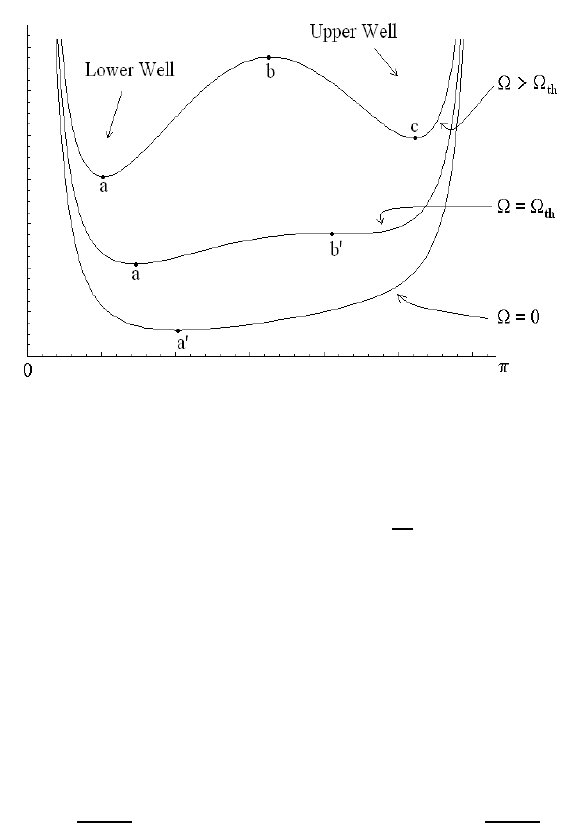
Figure 3.6: Effective potential of the charged pendulum in a magnetic field
Figure 3.6 shows the dimensionless effective potential
V (θ) for α = 1 and several values
of the dimensionless parameter Ω. When Ω is below the threshold value Ω
th
=1.94204...
(for α = 1), the effective potential has a single local minimum (point a
0
in Figure 3.6).
At threshold (Ω = Ω
th
), an inflection point develops at point b
0
. Above this threshold
(Ω > Ω
th
), a local maximum (at p oint b) and two local minima (at points a and c) appear.
Note that the local maximum at point b implies the existence of a separatrix solution,
which separates the bounded motion in the lower well and the upper well.
The normalized Euler-Lagrange equations are
ϕ
0
=Ω+
α
sin
2
θ
and θ
00
+ sin θ = sin θ cos θ
α
2
sin
4
θ
− Ω
2
!
where τ = ω
g
t denotes the dimensionless time parameter and the dimensionless parameters
are defined in terms of physical constants.
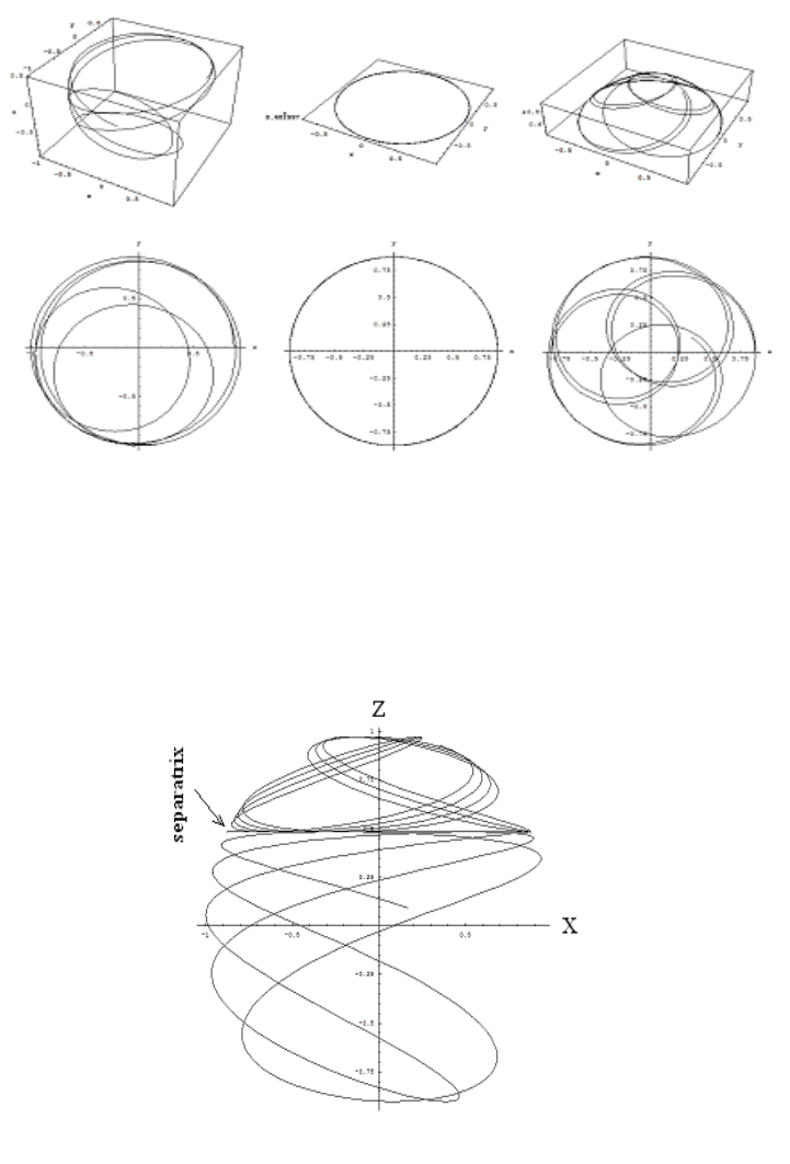
Figures 3.7 below show three-dimensional spherical projections (first row) and (x, y)-
plane projections (second row) for three cases above threshold (Ω > Ω
th
): motion in the
lower well (left column), separatrix motion (center column), and motion in the upper
well (right column). Figure 3.8 shows the (x, z)-plane projections for these three cases
combined on the same graph. These Figures clearly show that a separatrix solution exists
which separates motion in either the upper well or the lower well.
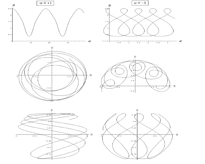
The equation for ϕ
0
does not change sign if α>−Ω, while its sign can change if
α<−Ω (or p
ϕ
< −m`
2
ω
c
). Figures 3.9 show the effect of changing α →−α by showing
the graphs θ versus ϕ (first row), the (x, y)-plane projections (second row), and the (x, z)-
plane projections (third row). One can clearly observe the wonderfully complex dynamics
62 CHAPTER 3. HAMILTONIAN MECHANICS
Figure 3.7: Orbits of the charged pendulum
Figure 3.8: Orbit projections
3.6. CHARGED SPHERICAL PENDULUM IN A MAGNETIC FIELD* 63
Figure 3.9: Retrograde motion
64 CHAPTER 3. HAMILTONIAN MECHANICS
of the charged pendulum in a uniform magnetic field, which is explicitly characterized by
the effective potential V (θ) given by Eq. (3.30).