Brealey, Myers. Principles of Corporate Finance. 7th edition

Подождите немного. Документ загружается.

Brealey−Meyers:

Principles of Corporate

Finance, Seventh Edition

VI. Options 21. Valuing Options

Companies, 2003

Notice that the payoffs from the levered investment in the stock are identical to

the payoffs from the call option. Therefore, both investments must have the same

value:

Presto! You’ve valued a call option.

To value the AOL option, we borrowed money and bought stock in such a way

that we exactly replicated the payoff from a call option. This is called a replicating

portfolio. The number of shares needed to replicate one call is called the hedge ra-

tio or option delta. In our AOL example one call is replicated by a levered position

in .5714 shares. The option delta is, therefore, .5714.

How did we know that AOL’s call option was equivalent to a levered position

in .5714 shares? We used a simple formula that says

You have learned not only to value a simple option but also that you can repli-

cate an investment in the option by a levered investment in the underlying asset.

Thus, if you can’t buy or sell an option on an asset, you can create a homemade op-

tion by a replicating strategy—that is, you buy or sell delta shares and borrow or

lend the balance.

Risk-Neutral Valuation Notice why the AOL call option should sell for $8.32. If

the option price is higher than $8.32, you could make a certain profit by buying

.5714 shares of stock, selling a call option, and borrowing $23.11. Similarly, if the

option price is less than $8.32, you could make an equally certain profit by selling

.5714 shares, buying a call, and lending the balance. In either case there would be

a money machine.

If there’s a money machine, everyone scurries to take advantage of it. So when

we said that the option price had to be $8.32 (or there would be a money machine),

we did not have to know anything about investor attitudes to risk. The option price

cannot depend on whether investors detest risk or do not care a jot.

This suggests an alternative way to value the option. We can pretend that all in-

vestors are indifferent about risk, work out the expected future value of the option

in such a world, and discount it back at the risk-free interest rate to give the cur-

rent value. Let us check that this method gives the same answer.

If investors are indifferent to risk, the expected return on the stock must be equal

to the risk-free rate of interest:

We know that AOL stock can either rise by 33 percent to $73.33 or fall by 25 percent

to $41.25. We can, therefore, calculate the probability of a price rise in our hypo-

thetical risk-neutral world:

⫽ 2.0 percent

⫹ 311 ⫺ probability of rise2 ⫻ 1⫺2524

Expected return ⫽ 3probability of rise ⫻ 334

Expected return on AOL stock ⫽ 2.0% per six months

Option delta ⫽

spread of possible option prices

spread of possible share prices

⫽

18.33 ⫺ 0

73.33 ⫺ 41.25

⫽ .5714

⫽155 ⫻ .57142 ⫺ 23.11 ⫽ $8.32

Value of call ⫽ value of .5714 shares ⫺ $23.11

bank loan

CHAPTER 21 Valuing Options 593

Of course, you don’t get seriously rich by dealing in .5714 shares. But if you multiply each of our trans-

actions by a million, it begins to look like real money.

Brealey−Meyers:

Principles of Corporate

Finance, Seventh Edition

VI. Options 21. Valuing Options

Companies, 2003

Therefore,

Notice that this is not the true probability that AOL stock will rise. Since investors

dislike risk, they will almost surely require a higher expected return than the risk-

free interest rate from AOL stock. Therefore the true probability is greater than .463.

We know that if the stock price rises, the call option will be worth $18.33; if it

falls, the call will be worth nothing. Therefore, if investors are risk-neutral, the ex-

pected value of the call option is

And the current value of the call is

Exactly the same answer that we got earlier!

We now have two ways to calculate the value of an option:

1. Find the combination of stock and loan that replicates an investment in the

option. Since the two strategies give identical payoffs in the future, they

must sell for the same price today.

2. Pretend that investors do not care about risk, so that the expected return on

the stock is equal to the interest rate. Calculate the expected future value of

the option in this hypothetical risk-neutral world and discount it at the risk-

free interest rate.

Valuing the AOL Put Option

Valuing the AOL call option may well have seemed like pulling a rabbit out of a

hat. To give you a second chance to watch how it is done, we will use the same

method to value another option—this time, the six-month AOL put option with a

$55 exercise price.

We continue to assume that the stock price will either rise to

$73.33 or fall to $41.25.

Expected future value

1 ⫹ interest rate

⫽

8.49

1.02

⫽ $8.32

⫽ $8.49

⫽ 1.463 ⫻ 18.332 ⫹ 1.537 ⫻ 02

3Probability of rise ⫻ 18.334 ⫹ 311 ⫺ probability of rise2 ⫻ 04

Probability of rise ⫽ .463, or 46.3%

594 PART VI Options

The general formula for calculating the risk-neutral probability of a rise in value is

In the case of AOL stock

In Chapter 9 we showed how you can value an investment either by discounting the expected cash

flows at a risk-adjusted discount rate or by adjusting the expected cash flows for risk and then dis-

counting these certainty-equivalent flows at the risk-free interest rate. We have just used this second

method to value the AOL option. The certainty-equivalent cash flows on the stock and option are the

cash flows that would be expected in a risk-neutral world.

When valuing American put options, you need to recognize the possibility that it will pay to exercise

early. We discuss this complication later in the chapter, but it is not relevant for valuing the AOL put

and we ignore it here.

p ⫽

.02 ⫺ 1⫺.252

.33 ⫺ 1⫺.252

⫽ .463

p ⫽

interest rate ⫺ downside change

upside change ⫺ downside change

Brealey−Meyers:

Principles of Corporate

Finance, Seventh Edition

VI. Options 21. Valuing Options

Companies, 2003

If AOL’s stock price rises to $73.33, the option to sell for $55 will be worthless. If

the price falls to $41.25, the put option will be worth . Thus

the payoffs to the put are

$55 ⫺ 41.25 ⫽ $13.75

CHAPTER 21

Valuing Options 595

1 put option $13.75 $0

Stock Price ⫽ $73.33Stock Price ⫽ $41.25

We start by calculating the option delta using the formula that we presented above:

Notice that the delta of a put option is always negative; that is, you need to sell delta

shares of stock to replicate the put. In the case of the AOL put you can replicate the

option payoffs by selling .4286 AOL shares and lending $30.81. Since you have sold

the share short, you will need to lay out money at the end of six months to buy it

back, but you will have money coming in from the loan. Your net payoffs are ex-

actly the same as the payoffs you would get if you bought the put option:

Option delta ⫽

spread of possible option prices

spread of possible stock prices

⫽

0 ⫺ 13.75

73.33 ⫺ 41.25

⫽⫺.4286

The delta of a put option is always equal to the delta of a call option with the same exercise price mi-

nus one. In our example, delta of .

Reminder: This formula applies only when the two options have the same exercise price and exercise date.

put ⫽ .5714 ⫺ 1 ⫽⫺.4286

Sale of .4286 shares

Repayment of

Total payoff $13.75 $ 0

⫹31.43⫹31.43loan ⫹ interest

⫺$31.43⫺$17.68

Stock Price ⫽ $73.33Stock Price ⫽ $41.25

Since the two investments have the same payoffs, they must have the same value:

Valuing the Put Option by the Risk-Neutral Method Valuing the AOL put option

with the risk-neutral method is a cinch. We already know that the probability of a

rise in the stock price is .463. Therefore the expected value of the put option in a

risk-neutral world is

And therefore the current value of the put is

The Relationship between Call and Put Prices We pointed out earlier that for Eu-

ropean options there is a simple relationship between the value of the call and that

of the put:

Value of put ⫽ value of call ⫺ share price ⫹ present value of exercise price

Expected future value

1 ⫹ interest rate

⫽

7.38

1.02

⫽ $7.24

⫽ $7.38

⫽ 1.463 ⫻ 02 ⫹ 1.537 ⫻ 13.752

3Probability of rise ⫻ 04 ⫹ 311 ⫺ probability of rise2 ⫻ 13.754

⫽ ⫺ 1.4286 ⫻ 552 ⫹ 30.81 ⫽ $7.24

Value of put ⫽⫺.4286

shares ⫹ $30.81 bank loan

Brealey−Meyers:

Principles of Corporate

Finance, Seventh Edition

VI. Options 21. Valuing Options

Companies, 2003

Since we had already calculated the value of the AOL call, we could also have used

this relationship to find the value of the put:

Everything checks.

Value of put ⫽ 8.32 ⫺ 55 ⫹

1.02

⫽ $7.24

596 PART VI Options

21.2 THE BINOMIAL METHOD FOR VALUING OPTIONS

The essential trick in pricing any option is to set up a package of investments in the

stock and the loan that will exactly replicate the payoffs from the option. If we can

price the stock and the loan, then we can also price the option. Equivalently, we can

pretend that investors are risk-neutral, calculate the expected payoff on the option

in this fictitious risk-neutral world, and discount by the rate of interest to find the

option’s present value.

These concepts are completely general, but there are several ways to find the

replicating package of investments. The example in the last section used a sim-

plified version of what is known as the binomial method. The method starts by

reducing the possible changes in next period’s stock price to two, an “up” move

and a “down” move. This simplification is OK if the time period is very short,

so that a large number of small moves is accumulated over the life of the option.

But it was fanciful to assume just two possible prices for AOL stock at the end

of six months.

We could make the AOL problem a trifle more realistic by assuming that there

are two possible price changes in each three-month period. This would give a

wider variety of six-month prices. And there is no reason to stop at three-month

periods. We could go on to take shorter and shorter intervals, with each interval

showing two possible changes in AOL’s stock price and giving an even wider se-

lection of six-month prices.

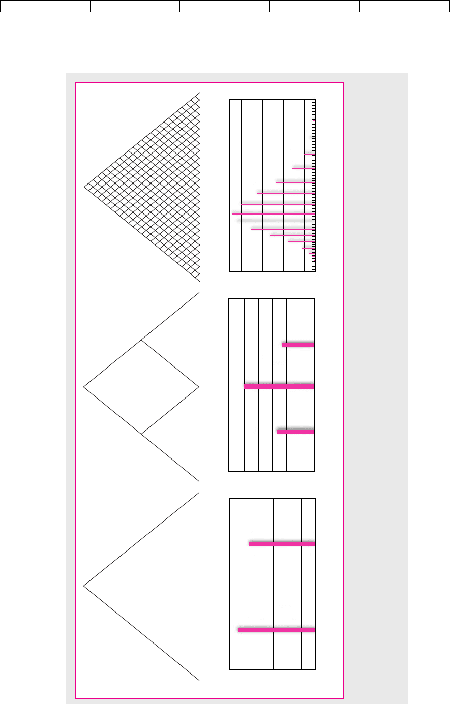
This is illustrated in Figure 21.1. The two left-hand diagrams show our start-

ing assumption: just two possible prices at the end of six months. Moving to the

right, you can see what happens when there are two possible price changes

every three months. This gives three possible stock prices when the option ma-

tures. In Figure 21.1(c) we have gone on to divide the six-month period into 26

weekly periods, in each of which the price can make one of two small moves.

The distribution of prices at the end of six months is now looking much more

realistic.

We could continue in this way to chop the period into shorter and shorter inter-

vals, until eventually we would reach a situation in which the stock price is chang-

ing continuously and there is a continuum of possible future stock prices.

Example: The Two-Stage Binomial Method

Dividing the period into shorter intervals doesn’t alter the basic method for valu-

ing a call option. We can still replicate the call by a levered investment in the stock,

but we need to adjust the degree of leverage at each stage. We will demonstrate

first with our simple two-stage case in Figure 21.1 (b). Then we will work up to the

situation where the stock price is changing continuously.

Brealey−Meyers:

Principles of Corporate

Finance, Seventh Edition

VI. Options 21. Valuing Options

Companies, 2003

597

–25 +33

Probability %

Percent price changes

(a) Percent price changes

–25 0 +33

–33 0 +50

+22.6⫺18.4

Probability %

Percent price changes

(b) Percent price changes

–33 0 +50

–77 –74 –71 –68 –64 –59 –55 –49 –43 –36 –29 –20 –11 4 12 25 40 57 76 97 120 147 176 209 246 287 334

–20–11 4 2512 40 57 76 97 120 147

Probability %

Percent price changes

FIGURE 21.1

This figure shows the possible six-month price changes for AOL stock assuming that the stock makes a single up or down move each six months [Fig. 21.1(a)], each

three months [Fig. 21.1(b)], or each week [Fig. 21.1(c)]. Beneath each tree we show a histogram of the possible six-month price changes, assuming investors are risk-

neutral.

Brealey−Meyers:

Principles of Corporate

Finance, Seventh Edition

VI. Options 21. Valuing Options

Companies, 2003

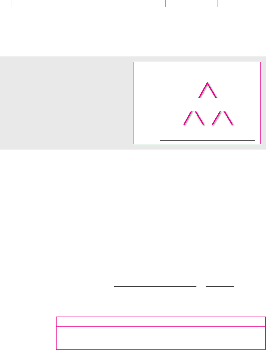
Figure 21.2 is taken from Figure 21.1 (b) and shows the possible prices of AOL

stock, assuming that in each three-month period the price will either rise by 22.6

percent or fall by 18.4 percent. We show in parentheses the possible values at

maturity of a six-month call option with an exercise price of $55. For example, if

AOL’s stock price turns out to be $36.62 in month 6, the call option will be

worthless; at the other extreme, if the stock value is $82.67, the call will be worth

. We haven’t worked out yet what the option will be worth

before maturity, so we just put question marks there for now.

Option Value in Month 3 To find the value of AOL’s option today, we start by

working out its possible values in month 3 and then work back to the present. Sup-

pose that at the end of three months the stock price is $67.43. In this case investors

know that, when the option finally matures in month 6, the stock price will be ei-

ther $55 or $82.67, and the corresponding option price will be $0 or $27.67. We can

therefore use our simple formula to find how many shares we need to buy in

month 3 to replicate the option:

Now we can construct a leveraged position in delta shares that would give iden-

tical payoffs to the option:

Option delta ⫽

spread of possible option prices

spread of possible stock prices

⫽

27.67 ⫺ 0

82.67 ⫺ 55

⫽ 1.0

$82.67 ⫺ $55 ⫽ $27.67

598 PART VI Options

Month 6 Stock Month 6 Stock

Buy 1.0 shares $55 $82.67

Borrow PV(55) ⫺55 ⫺55

Total payoff $ 0 $27.67

Price ⫽ $82.67Price ⫽ $55

$55.00

(?)

Now

$82.67

($27.67)

$36.62

($0)

$55.00

($0)

Month 6

Month 3

$67.43

(?)

$44.88

(?)

FIGURE 21.2

Present and possible future prices of AOL stock assuming

that in each three-month period the price will either rise

by 22.6% or fall by 18.4%. Figures in parentheses show

the corresponding values of a six-month call option with

an exercise price of $55.

Since this portfolio provides identical payoffs to the option, we know that the value

of the option in month 3 must be equal to the price of 1 share less the $55 loan dis-

counted for 3 months at 4 percent per year, about 1 percent for 3 months:

Therefore, if the share price rises in the first three months, the option will be worth

$12.97. But what if the share price falls to $44.88? In that case the most that you can

Value of call in month 3 ⫽ $67.43 ⫺ $55/1.01 ⫽ $12.97

Brealey−Meyers:

Principles of Corporate

Finance, Seventh Edition

VI. Options 21. Valuing Options

Companies, 2003

CHAPTER 21 Valuing Options 599

hope for is that the share price will recover to $55. Therefore the option is bound to

be worthless when it matures and must be worthless at month 3.

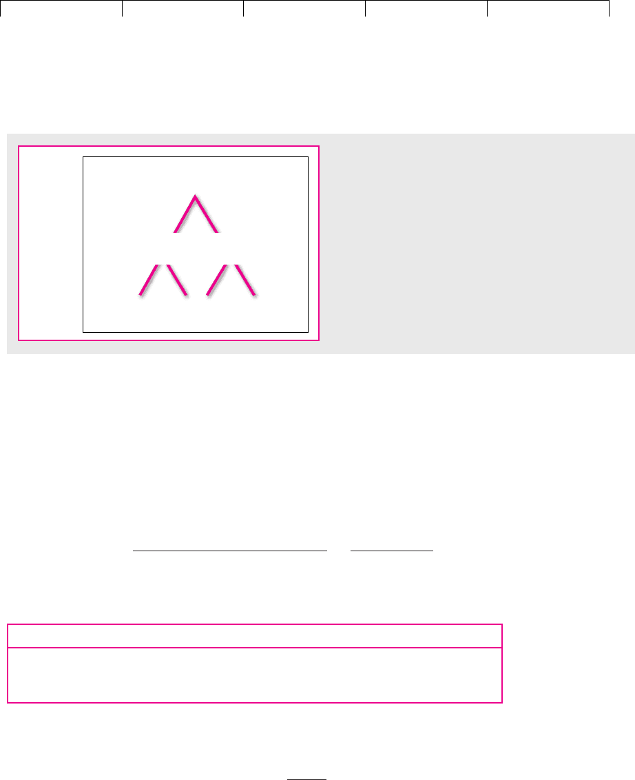
Option Value Today We can now get rid of two of the question marks in Figure

21.2. Figure 21.3 shows that if the stock price in month 3 is $67.43, the option value

is $12.97 and, if the stock price is $44.88, the option value is zero. It only remains to

work back to the option value today.

We again begin by calculating the option delta:

We can now find the leveraged position in delta shares that would give identical

payoffs to the option:

Option delta ⫽

spread of possible option prices

spread of possible stock prices

⫽

12.97 ⫺ 0

67.43 ⫺ 44.88

⫽ .575

$55.00

(?)

Now

$82.67

($27.67)

$36.62

($0)

$55.00

($0)

Month 6

Month 3

$67.43

($12.97)

$44.88

($0)

FIGURE 21.3

Present and possible future prices of AOL stock. Figures

in parentheses show the corresponding values of a six-

month call option with an exercise price of $55.

Month 3 Stock Month 3 Stock

Buy .575 shares $25.81 $38.78

Borrow PV(25.81) ⫺25.81 ⫺25.81

Total payoff $ 0 $12.97

Price ⫽ $67.43Price ⫽ $44.88

The value of the AOL option today is equal to the value of this leveraged position:

The General Binomial Method

Moving to two steps when valuing the AOL call probably added extra realism. But

there is no reason to stop there. We could go on, as in Figure 21.1, to chop the pe-

riod into smaller and smaller intervals. We could still use the binomial method to

work back from the final date to the present. Of course, it would be tedious to do

the calculations by hand, but simple to do so with a computer.

Since a stock can usually take on an almost limitless number of future values, the

binomial method gives a more realistic and accurate measure of the option’s value if

⫽ .575 ⫻ $55 ⫺

$25.81

1.01

⫽ $6.07

PV option ⫽ PV1.575 shares2 ⫺ PV1$25.812

Brealey−Meyers:

Principles of Corporate

Finance, Seventh Edition

VI. Options 21. Valuing Options

Companies, 2003

600 PART VI Options

we work with a large number of subperiods. But that raises an important question.

How do we pick sensible figures for the up and down changes in value? For exam-

ple, why did we pick figures of percent and percent when we revalued

AOL’s option with two subperiods? Fortunately, there is a neat little formula that re-

lates the up and down changes to the standard deviation of stock returns:

where

for natural

deviation of (continuously compounded) stock returns

as fraction of a year

When we said that AOL’s stock could either rise by 33.3 percent or fall by 25 per-

cent over six months , our figures were consistent with a figure of 40.69 per-

cent for the standard deviation of annual returns:

To work out the equivalent upside and downside changes when we divide the pe-

riod into two three-month intervals (h ⫽ .25) , we use the same formula:

The center columns in Table 21.1 show the equivalent up and down moves in the

value of the firm if we chop the period into monthly or weekly periods, and the fi-

nal column shows the effect on the estimated option value. (We will explain the

Black–Scholes value shortly.)

The Binomial Method and Decision Trees

Calculating option values by the binomial method is basically a process of solving

decision trees. You start at some future date and work back through the tree to the

present. Eventually the possible cash flows generated by future events and actions

are folded back to a present value.

Is the binomial method merely another application of decision trees, a tool of

analysis that you learned about in Chapter 10? The answer is no, for at least two

1 ⫹ downside change ⫽ d ⫽ 1/u ⫽ 1/1.226 ⫽ .816

1 ⫹ upside change 13-month interval2 ⫽ u ⫽ e

.40692.25

⫽ 1.226

1 ⫹ downside change ⫽ d ⫽ 1/u ⫽ 1/1.333 ⫽ .75

1 ⫹ upside change 16-month interval2 ⫽ u ⫽ e

.40692.5

⫽ 1.333

1h ⫽ .52

h ⫽ interval

␴ ⫽ standard

logarithms ⫽ 2.718e ⫽ base

1 ⫹ downside change ⫽ d ⫽ 1/u

1 ⫹ upside change ⫽ u ⫽ e

␴2h

⫺18.4⫹22.6

Intervals in

Change per Interval (%)

Estimated Option

a Year (1/h) Upside Downside Value

2 $8.32

4 6.07

12 6.65

52 6.75

Black–Scholes value ⫽ $6.78

⫺5.5⫹ 5.8

⫺11.1⫹12.4

⫺18.4⫹22.6

⫺25.0⫹33.3

TABLE 21.1

As the number of intervals is

increased, you must adjust the range

of possible changes in the value of the

asset to keep the same standard

deviation. But you will get increasingly

close to the Black–Scholes value of the

AOL call option.

Note: The standard deviation is .␴ ⫽ .4069

Brealey−Meyers:

Principles of Corporate

Finance, Seventh Edition

VI. Options 21. Valuing Options

Companies, 2003

reasons. First, option pricing theory is absolutely essential for discounting

within decision trees. Standard discounting doesn’t work within decision trees

for the same reason that it doesn’t work for puts and calls. As we pointed out in

Section 21.1, there is no single, constant discount rate for options because the

risk of the option changes as time and the price of the underlying asset change.

There is no single discount rate inside a decision tree, because if the tree contains

meaningful future decisions, it also contains options. The market value of the fu-

ture cash flows described by the decision tree has to be calculated by option

pricing methods.

Second, option theory gives a simple, powerful framework for describing

complex decision trees. For example, suppose that you have the option to post-

pone an investment for many years. The complete decision tree would overflow

the largest classroom chalkboard. But now that you know about options, the op-

portunity to postpone investment might be summarized as “an American call on

a perpetuity with a constant dividend yield.” Of course, not all real problems

have such easy option analogues, but we can often approximate complex deci-

sion trees by some simple package of assets and options. A custom decision tree

may get closer to reality, but the time and expense may not be worth it. Most men

buy their suits off the rack even though a custom-made suit from Saville Row

would fit better and look nicer.

CHAPTER 21

Valuing Options 601

21.3 THE BLACK–SCHOLES FORMULA

Look back at Figure 21.1, which showed what happens to the distribution of pos-

sible AOL stock price changes as we divide the option’s life into a larger and larger

number of increasingly small subperiods. You can see that the distribution of price

changes becomes increasingly smooth.

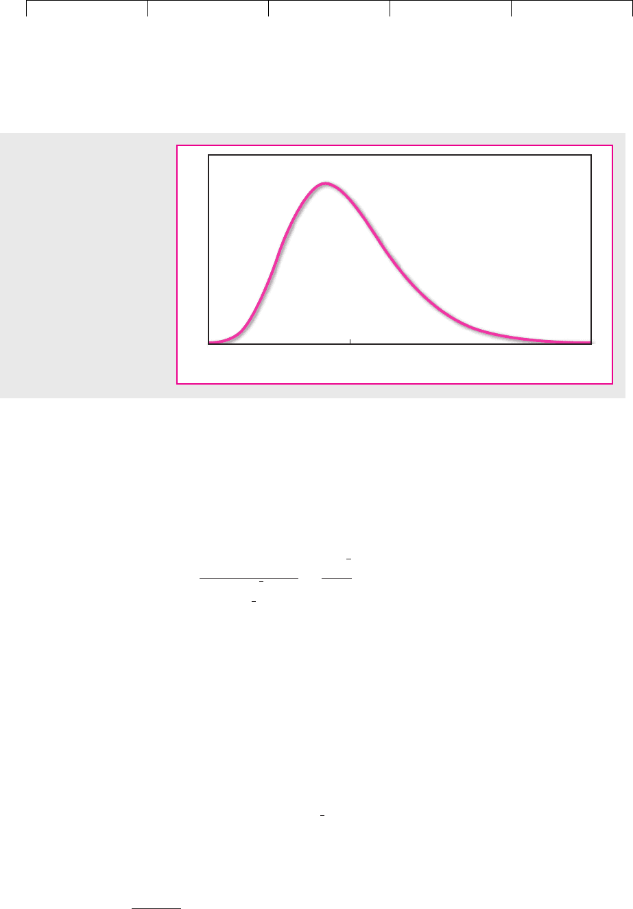
If we continued to chop up the option’s life in this way, we would eventually

reach the situation shown in Figure 21.4, where there is a continuum of possible

stock price changes at maturity. Figure 21.4 is an example of a lognormal distribu-

tion. The lognormal distribution is often used to summarize the probability of dif-

ferent stock price changes.

It has a number of good commonsense features. For

example, it recognizes the fact that the stock price can never fall by more than 100

percent, but that there is some, perhaps small, chance that it could rise by much

more than 100 percent.

Subdividing the option life into indefinitely small slices does not affect the

principle of option valuation. We could still replicate the call option by a levered

investment in the stock, but we would need to adjust the degree of leverage con-

tinuously as time went by. Calculating option value when there is an infinite

number of subperiods may sound a hopeless task. Fortunately, Black and Scholes

derived a formula that does the trick. It is an unpleasant-looking formula, but on

When we first looked at the distribution of stock price changes in Chapter 8, we assumed that these

changes were normally distributed. We pointed out at the time that this is an acceptable approximation

for very short intervals, but the distribution of changes over longer intervals is better approximated by

the lognormal.

Brealey−Meyers:

Principles of Corporate

Finance, Seventh Edition

VI. Options 21. Valuing Options

Companies, 2003

602 PART VI Options

closer acquaintance you will find it exceptionally elegant and useful. The for-

mula is

↑↑ ↑

3N(d

) ⫻ P4 ⫺ 3N(d

) ⫻ PV(EX)4

where

normal probability density function

price of option; PV(EX) is calculated by discounting at the

risk-free interest rate

of periods to exercise date

of stock now

deviation per period of (continuously compounded) rate of

return on stock

Notice that the value of the call in the Black–Scholes formula has the same proper-

ties that we identified earlier. It increases with the level of the stock price P and de-

creases with the present value of the exercise price PV(EX), which in turn depends

on the interest rate and time to maturity. It also increases with the time to maturity

and the stock’s variability .

To derive their formula Black and Scholes assumed that there is a continuum

of stock prices, and therefore to replicate an option investors must continu-

ously adjust their holding in the stock. Of course this is not literally possible,

1␴2t

␴ ⫽ standard

P ⫽ price

t ⫽ number

EX ⫽ exercise

N1d2 ⫽ cumulative

⫽ d

⫺ ␴2t

⫽

log 3P/PV1EX24

␴2t

⫹

␴2t

Value of call option ⫽ 3delta ⫻ share price4 ⫺ 3bank loan4

Probability

Percent price changes

–70 0 +130

FIGURE 21.4

As the option’s life is divided

into more and more sub-

periods, the distribution of

possible stock price changes

approaches a lognormal

distribution.

That is, N(d) is the probability that a normally distributed random variable

x will be less than or equal

to d. in the Black–Scholes formula is the option delta. Thus the formula tells us that the value of

a call is equal to an investment of in the common stock less borrowing of .N1d

2 ⫻ PV1EX2N1d

N1d