Biringen S., Chow C.-Y. An Introduction to Computational Fluid Mechanics by Example

Подождите немного. Документ загружается.

192 VISCOUS FLUID FLOWS

y/h

−1

= [1 − (y/h)

]

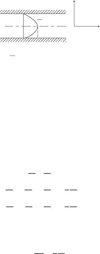
FIGURE 3.8.2 Schematic of plane Poiseuille ﬂow.

problem will consist of perturbing the laminar, steady, fully developed ﬂow in the

channel (Figure 3.8.2) with small amplitude disturbances in the form of traveling

waves and determining the conditions under which these disturbances (normal

modes) will amplify and eventually drive the laminar base ﬂow to a turbulent

state. The steady-state solution (base ﬂow) for this pressure-driven ﬂow is called

the Poiseuille ﬂow and generates a parabolic velocity proﬁle between the two

plates (Figure 3.8.2). This solution is obtained from the governing equations

written for the two-dimensional ﬂow of an incompressible ﬂuid. Note that, in

compliance with customary notation, for this problem we deﬁne the vertical

axis as the y axis and consequently the plates are located at y =±h,whereh

is the channel half-height. The continuity, x-momentum and the y-momentum

equations are given as

∂u

∂x

∂v

∂y

= 0 (3.8.26)

∂u

∂t

∂u

∂x

∂u

∂y

=−

∂p

∂x

+ν∇

u (3.8.27)

∂v

∂t

∂v

∂x

∂v

∂y

=−

∂p

∂y

+ν∇

v (3.8.28)

We assume that the ﬂow is driven by a constant mean pressure gradient along the

x direction, where u = u(y) only. Then, for steady ﬂow, (3.8.26) and (3.8.28)

are identically zero, and (3.8.27) reduces to

y =±h, u = 0

(3.8.29)

Integrating twice and imposing the boundary conditions, one obtains

U = (1 − y

), −1 ≤ y ≤ 1 (3.8.30)

Here, U is nondimensionalized by the channel centerline velocity, U

−(h

/2ρν)(dp/dx),andx and y are nondimensionalized by h. Equation

(3.8.30) is the laminar base ﬂow, which will be perturbed by the imposed

disturbances. A similar solution is given in Section 3.6.

FLOW STABILITY AND PSEUDO-SPECTRAL METHODS 193

In a similar manner as in the previous example, it is assumed that the velocity

components and the pressure can be written as a sum of a mean (base) component

and a small amplitude ﬂuctuating disturbance component:

u = U (y) + ˆu(x, y, t),

v = ˆv(x, y, t),

p = P(x) + ˆp(x, y, t)

(3.8.31)

Substituting (3.8.31) into (3.8.26)–(3.8.28) and subtracting the base ﬂow (3.8.29),

and, further, linearizing the equations with respect to the quadratic terms in the

ﬂuctuating components and scaling the pressure with density, one obtains

∂ ˆu

∂x

∂ ˆv

∂y

= 0 (3.8.32)

∂ ˆu

∂t

∂ ˆu

∂x

∂U

∂y

∂ ˆp

∂x

= ν



∂

ˆu

∂x

∂

ˆu

∂y



(3.8.33)

∂ ˆv

∂t

∂ ˆv

∂x

∂ ˆp

∂y

= ν



∂

ˆv

∂x

∂

ˆv

∂y



(3.8.34)

where ˆp is kinematic pressure, or pressure divided by density, ρ. Noting that

because these equations are linear, separation of variables can be used and a

solution of the following form can be assumed:

ˆu(x, y, t) =˜u(y)e

I α(x−ct)

ˆv(x, y, t) =˜v(y)e

I α(x−ct)

ˆp(x, y, t) =˜p(y)e

I α(x−ct)

(3.8.35)

In (3.8.35), assuming temporal growth of the disturbances, the wave number α

is a real positive number but the wave velocity c is complex. The real part c

corresponds to the phase velocity, and the imaginary part c

is the growth rate of

the disturbances. Hence, for c

< 0, disturbances attenuate; c

= 0 gives the neu-

tral curve; and c

> 0 corresponds to amplifying disturbances, which are called

the Tollmien-Schlichting waves. Substituting (3.8.35) into (3.8.32)–(3.8.34), after

elimination of the exponential factors, we obtain the following equations:

I α ˜u +˜v



= 0 (3.8.36)

I α(U −c) ˜u +˜vU



+I α ˜p = ν(˜u



−α

˜u) (3.8.37)

I α(U −c) ˜v +˜p



= ν(˜v



−α

˜v) (3.8.38)

In these equations primes denote differentiation with respect to y.Next, ˜u and

˜p are eliminated from (3.8.38) by using (3.8.36) and (3.8.37), and the resulting

equation is nondimensionalized by the channel half-height h and the channel

194 VISCOUS FLUID FLOWS

centerline velocity U

. The resulting equation is the fourth-order, linear Orr-

Sommerfeld equation, which governs the stability of parallel shear ﬂows and

reads (with all the variables in nondimensional form)

(U −c)(v



−α

v) − vU



=−

α Re





−2α



+α



For Poiseuille ﬂow, (3.8.39)

Re =

, U = (1 − y

), U



=−2, v

y=±1

= 0, v



y=±1

= 0

Equation (3.8.39) shows that both the Orr-Sommerfeld equation and its bound-

ary conditions are homogeneous, and the temporal problem is reduced to an

eigenvalue problem with the following functional form:

f (Re, α, c

, c

) = 0 (3.8.40)

Then, for given real α and Re, the computational problem is to calculate the

complex eigenvalue, c.

A very efﬁcient and accurate method to solve the eigenvalue problem (3.8.39)

is the use of spectral methods (or transform methods) with Chebyshev differ-

entiation matrices. The use of these methods for linear stability problems and

for the Navier-Stokes equations has been pioneered by Orszag’s (1971) work

on Poiseuille ﬂow; practical aspects and applications have been exposed by two

exceptionally well-written books by Trefethen (2000) and Moin (2001). Tre-

fethen’s book contains short and very efﬁciently written MATLAB codes, which

will form the basis of the solution procedure that we will use in this section to

solve (3.8.39). Comprehensive coverage of advanced methods based on spectral

elements can be found in Karniadakis and Sherwin (2005).

For nonperiodic functions over an interval [−1, 1], derivatives can be calcu-

lated by an interpolation polynomial at Chebyshev points obtained from

= cos( j π/N ), j = 0, 1, ..., N (3.8.41)

These points are unequally distributed within the computational domain and are

clustered toward the boundaries at y =±1 (with grid index j = 0ony = 1,

and the grid index j = N on y =−1) and are particularly suitable for problems

where gradients of the ﬂow-ﬁeld variables are very strong at the boundaries,

such as in wall-bounded ﬂows. We also note that these points correspond to

the extrema of the Chebyshev polynomial, T

(y),wherek indicates the degree

of the polynomial. These polynomials can be used to approximate any func-

tion and its derivatives at the Chebyshev points (3.8.41). It is important to

consider that spectral accuracy, which can be expressed in terms of the expo-

nentially decreasing error, i.e., ε ∼ e

−N

, will be achieved with k > 16 for most

problems.

FLOW STABILITY AND PSEUDO-SPECTRAL METHODS 195

The kth degree Chebyshev polynomial is deﬁned as

(y) = cos(k cos

−1

y) ≡ cos(kθ) (3.8.42)

Then, using trigonometric identities, we obtain

(y) = 1

(y) = y

(y) = 2y

−1

(y) = 4y

−3y

k+1

(y) = 2yT

(y) −T

k−1

(y) k ≥ 1

(3.8.43)

The Chebyshev polynomial T

(y) has N zeros in the interval [−1, 1] located at

= cos



π(j − 1/2)



, j = 1, 2, ..., N (3.8.44)

In the same interval, it has (N + 1) extrema at locations given by (3.8.41). From

approximation theory, using the orthogonality of the polynomials (Moin, 2001,

p. 180), any function can be expanded in terms of Chebyshev polynomials at

collocation points given by (3.8.41), by a given set of coefﬁcients,

u(y) =



k=0

(y), (3.8.45)

where a

is the coefﬁcient for the kth Chebyshev polynomial.

As an example, let us consider the function u(y) = y

. Using (3.8.45), we can

write

u(y) = a

(y) +a

(y) +···

(y) = 1, T

(y) = y, T

(y) = 2y

−1 (3.8.46)

∴ a

= 0.5, a

= 0, a

= 0.5

Equation (3.8.45) can be written in discrete form such that

= u(y

) =



k=0

), j = 0, 1, ..., N (3.8.47)

196 VISCOUS FLUID FLOWS

Similarly,



j=0

, k = 0, 1, ..., N



2 j = 0, N

1otherwise

(3.8.48)

We can write this expression in matrix form for the Chebyshev coefﬁcient vec-

tor, a:

a =

Tu (3.8.49)

Here, the vector of unknowns contains the values of u(y

) at the Chebyshev

collocation points. In a similar fashion, we can obtain the derivative



) =



k=0

) (3.8.50)

Equation (3.8.50) can be written in vector–matrix form:



= Tb (3.8.51)

Vectors a and b are related through the matrix G (Moin, 2001, p. 187),

b = Ga

⎧

⎪

⎨

⎪

⎩

0ifk ≥ j or k + j even

otherwise

(3.8.52)

Hence, it follows that



= TGa = TG

Tu = Du (3.8.53)

Matrices T and

T are functions of the Chebyshev polynomials, and the elements,

,ofthe(N + 1) ×(N + 1) Chebyshev collocation differentiation matrix D are

given by (Gottlieb, Hussaini, Orszag, 1984; Trefethen, 2000; Moin, 2001)

, d

=−

−y

2(1 −y

)

, j = 1, 2, ..., (N − 1)

(−1)

j+k

−y

)

, j = k, j, k = 0, 1, ..., N

(3.8.54)

FLOW STABILITY AND PSEUDO-SPECTRAL METHODS 197

In (3.8.54), y

are the collocations points (grid points) obtained from (3.8.41)

and c

are given as



2, j = 0orN

1, otherwise

A remarkable feature of the Chebyshev differentiation matrix, D, is that higher-

order derivatives of the function u(y) can be directly calculated from its corre-

sponding powers:



= D



= D

(3.8.55)

Consider the boundary value problem,



(y) +π u(y) = π ; u(−1) = 0, u(+1) = 1 (3.8.56)

Evaluating u(y) at the Chebyshev collocation points (3.8.41), and using (3.8.55),

we get

Au = c

A ≡ (D

+πI)

c = π(diagI)

(3.8.57)

Note that the D matrix and, consequently, the A matrix are both written for all

the collocation points, including the boundary points; i.e., the ﬁrst and last rows

corresponding to the boundary points. The boundary conditions at y =±1 can

be implemented by modifying these rows:

⎡

⎢

⎣

10··· 00

1,0

1,1

··· a

1,N

N −1,0

··· a

N −1,N −1

N −1,N

00··· 01

⎤

⎥

⎦



 

⎡

⎢

⎣

N −1

⎤

⎥

⎦

⎡

⎢

⎣

⎤

⎥

⎦

(3.8.58)

In (3.8.58),

A is the A matrix modiﬁed by the implementation of the boundary

conditions. The solution of (3.8.57) can be obtained by the MATLAB backslash

division:

u =

A \ c



(3.8.59)

The backslash indicates LU factorization with left division of

A into c



and the

apostrophe transposes the row vector c into a column vector c



. Program 3.7 is

a MATLAB script that solves (3.8.56). In Fig. 3.8.3, computational results are

compared with the exact solution for (3.8.56), and shows that even with only nine

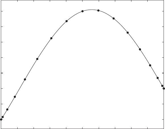
198 VISCOUS FLUID FLOWS

−1 −0.8 −0.6 −0.4 −0.2 0 0.2 0.4 0.6 0.8 1

0.5

1.5

2.5

3.5

u" + π u = π

FIGURE 3.8.3 Solution of (3.8.56) using the Chebyshev matrix method with 9 collocation

points. The solid line is the exact solution.

collocation points, the Chebyshev matrix method provides remarkably accurate

results. We should also note that in the MATLAB program, the indices for the

grid point locations run from 1 to (N +1), not from zero to N as in (3.8.41).

The solution of the hydrodynamic stability problem outlined above and given

by (3.8.39) and (3.8.40) can be obtained in a similar manner. For temporal eigen-

values, the wave number α, the Reynolds number Re, and the base velocity proﬁle

U (y) are all real and given, so that the unknowns in the problem are the complex

perturbation velocity, v, and the complex wave velocity, c

U (y) = 1 −y

, U



(y) =−2

v(y) = v

+I v

c = c

+Ic

(3.8.60)

We can deﬁne the various derivatives appearing in (3.8.39) in terms of the Cheby-

shev matrix:



= Dv, v



= D

v, v



= D

U = diag[U

···U

], y

=+1, y

=−1

(3.8.61)

FLOW STABILITY AND PSEUDO-SPECTRAL METHODS 199

Equation (3.8.39) can now be written as a generalized eigenvalue problem for

the complex wave velocity λ =−ic, and deﬁning I as the identity matrix

Av = λBv

A = (αRe)

−1



−2α

+α



−2II − I diag



1 − y



−α



B = D

−α

(3.8.62)

To implement the homogeneous boundary conditions, the ﬁrst and last rows

of the A matrix are modiﬁed as before (3.8.58), and the zero derivative boundary

condition (Neumann condition) at y = 1 is imposed by replacing the second row

of the A matrix with the ﬁrst row of the D matrix (Chebyshev matrix for the ﬁrst

derivative). We again note that in the MATLAB program, the indices for the grid

point locations will run from 1 to (N +1), not from zero to N . Consequently, to

impose the homogeneous Neumann boundary condition at y =−1, we replace

the N th row of the A matrix with the (N + 1)th row (last row) of the D matrix.

If we denote the modiﬁed matrices as

A and B, for given α and Re, the resulting

equation can be written as a generalized eigenvalue problem (3.8.62), where the

complex eigenvalue is λ, and the corresponding complex eigenfunction is v;the

solution will provide N eigenvalues and N corresponding eigenfunctions for each

eigenvalue, and we note that λ

> 0 indicates amplifying disturbance waves:

A − λB

v = 0 (3.8.63)

The solution for (3.8.63) can be obtained by the MATLAB function eig(A,B).

Program 3.8 is a MATLAB script that solves (3.8.62) for the full eigenvalue

spectrum with N = 100, and given different values of Re and α. The elements of

the D matrix are calculated by using a compact MATLAB program from Trefthen

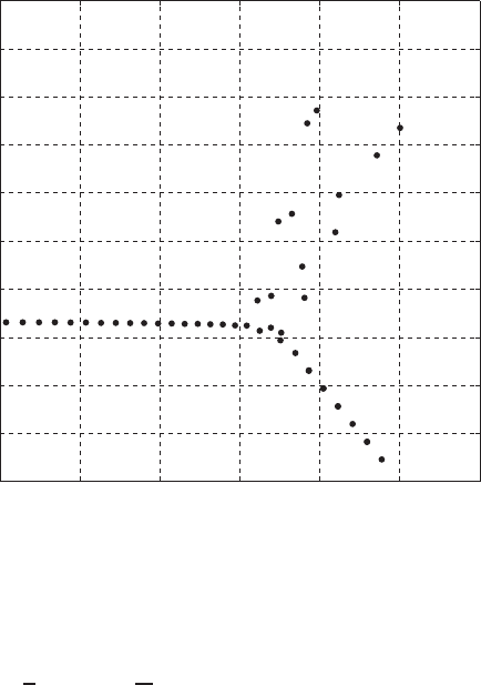
(2000, p. 54). Figure 3.8.4 illustrates the eigenvalue spectrum for Re = 5772, α =

1.02, which are the critical values for this ﬂow as calculated by Orszag (1971). For

this case (λ

)

max

=−0.0000004209 ≈ 0, representing a neutrally stable wave. If

we increase the Reynolds number to Re = 7500, we obtain (λ

)

max

= 0.002029

(Fig. 3.8.5), indicating that this disturbance wave will grow exponentially in time.

It is apparent that within the bounds of a stability limit, certain combinations of

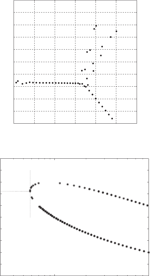
Re and α will result in unstable (growing) waves. This limit is called the neutral

stability curve and is calculated by setting λ

= 0, as shown in Fig. 3.8.6 for

Poiseuille ﬂow obtained by modifying Program 3.8. For a given Re  5800, there

is a narrow band of wave numbers (α values) that will resonate with the mean

velocity proﬁle and drive the laminar channel ﬂow to instability and, eventually,

to turbulence.

Problem 3.15 Modify Program 3.8. to obtain the neutral stability curve for

the general Couette ﬂow, which represents pressure-driven ﬂow in a channel

with the upper lid moving at a constant velocity, U

. The mean velocity proﬁle,

200 VISCOUS FLUID FLOWS

−1 −0.8 −0.6 −0.4 −0.2 0 0.2

−1

−0.9

−0.8

−0.7

−0.6

−0.5

−0.4

−0.3

−0.2

−0.1

Re = 5772 (λ

)

max

= −0.00000042086

FIGURE 3.8.4 Eigenvalues for plane channel ﬂow for α = 1.02, Re = 5772.

nondimensionalized with the wall velocity can be written as

U (y) =

(1 + y) +

(1 −y

), u = 0 y =±1 (3.8.64)

Obtain the neutral stability curves for B = 1, 3, 7, 25, 100. For larger B, does the

curve approach that of the pressure-driven channel (Poiseuille) ﬂow? Plot the

critical Reynolds number, Re

as a function of the Brinkman number B,and

comment on if the ﬂow becomes more or less stable when upper wall motion is

added. When B = 0, are there any unstable modes? The neutral stability curves

for different B should be obtained for 0 ≤ α ≤ 1.2, and 3.10

≤ Re ≤ 10

Pseudo-spectral or transform methods can also be very effective for problems

that are periodic in one or more space dimensions. Such problems occur in transi-

tional or turbulent ﬂow simulations; for example, in the pressure-driven channel

ﬂow, eigenfunctions obtained from the Orr-Sommerfeld solution can be used

as initial conditions for the numerical simulation of the Navier-Stokes equation

to investigate how the laminar ﬂow will become turbulent as the disturbance

amplitudes grow exponentially due to nonlinear interactions generated by the

convective terms. It is often preferable to assume the ﬂow to be periodic in the

streamwise x direction, and simply observe the time evolution of one period of

FLOW STABILITY AND PSEUDO-SPECTRAL METHODS 201

−1 −0.8 −0.6 −0.4 −0.2 0 0.2

−1

−0.9

−0.8

−0.7

−0.6

−0.5

−0.4

−0.3

−0.2

−0.1

Re = 7500 (λ

)

max

= −0.00202859625

FIGURE 3.8.5 Eigenvalues for plane channel ﬂow for α = 1.02, Re = 7500.

0.3

0.4

0.5

0.6

0.7

0.8

0.9

1.1

1.2

1.3

α, nondimensional wave number

Stable

(5772,1.02)

= 0

Unstable

FIGURE 3.8.6 Neutral stability curve (λ

= 0) for plane channel ﬂow.