Biringen S., Chow C.-Y. An Introduction to Computational Fluid Mechanics by Example

Подождите немного. Документ загружается.

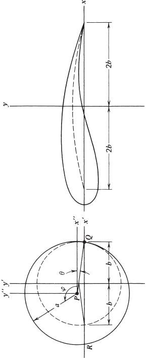
FIGURE 2.6.3 Mapping of two circles in the x



-y



plane into a circular arc and an airfoil in the x-y plane by the Joukowski transformation

z = z



INVERSE METHOD II: CONFORMAL MAPPING 83

In the computer program to be constructed, we will ﬁnd the coordinates of

points along some streamlines of the ﬂow before the mapping. This given ﬂow is

usually in a relatively simple form, and its characteristics are well known. Some

common examples are the uniform ﬂow and the ﬂow around a circle. These points

will be mapped according to the speciﬁed transformation and will be plotted on

the transformed plane. Such a plot will display the pattern of the transformed

ﬂow if the number of points is large. In a similar fashion the equipotential lines,

velocity, or pressure distribution of the transformed ﬂow may also be plotted.

Our illustrative example is concerned with a uniform ﬂow U in the positive x

direction past the Joukowski airfoil shown in Fig. 2.6.3. The airfoil is the image

in the x-y plane of the circle of radius a centered at the point P in the x



-y



plane

and, in particular, its sharp trailing edge at x = 2b is the image of the point Q

at x



= b. The ﬂow about the airfoil is obtained from the ﬂow of uniform speed

U past the circle using the transformation (2.6.19).

The magnitude of the velocity V in the x-y plane is related to that of V



the x



-y



plane through the equation



By the use of (2.6.9) and (2.6.19), it becomes

V =



1 −







(2.6.20)

This equation shows that the ﬂow speed at the trailing edge of the airfoil becomes

inﬁnite if the speed at Q (where z



= b) is of a ﬁnite magnitude. Physically such

a situation is not allowed. Based on observations of bodies with a sharp trailing

edge moving through a ﬂuid, the Kutta condition states that the ﬂow speed at the

trailing edge must be zero if the trailing-edge angle is ﬁnite, or the speed there

must be ﬁnite if the trailing-edge angle is zero. In the present case of a Joukowski

airfoil, the Kutta condition is fulﬁlled only when the speed at Q vanishes. In other

words, the airfoil will create about itself a clockwise circulation  whose strength

is just sufﬁcient to make the point Q a stagnation point on the circular cylinder

in the x



-y



plane. Let z



(= x



+iy



) be the position of the point P in the x



-y



plane and let θ be the angle between the line PQ and the direction of the free

stream, as indicated in Fig. 2.6.3. The magnitude of the circulation is (Kuethe

and Chow, 1998, Section 4.7)

 = 4πaU sin θ

Since sin θ = y



/a, this equation becomes

 = 4πy



U (2.6.21)

84 INVISCID FLUID FLOWS

The ﬂow about the circle is then constructed by adding to the uniform stream a

doublet and a line vortex. In the x



, y



coordinate system whose origin coincides

with P, the complex potential of the resultant ﬂow is

w = U



+i2y



log





%

(2.6.22)

where z



= x



+iy



, and a constant −i2y



log a has been added so that the value

of the stream function on the circle remains unchanged after the introduction of

the vortex. The complex potential can easily be expressed in terms of z



by using

the transformation



= z



−z



(2.6.23)

The shape of the airfoil is controlled by varying a, b and the coordinates

of the center P;a and b determine the thickness envelope and chord length,

respectively, while the height of P determines the maximum camber of the airfoil.

By inspecting Fig. 2.6.3, these variables are related through the equation

= y



+(b − x



)

For a given value of a, we may assume a set of values for two of the quantities

on the right-hand side of the previous equation, say, for b and y



, and compute

the value of the third, or



= b −

−y



(2.6.24)



must be negative to produce an airfoil having its sharp edge on the downstream

side, similar to the one shown in Fig. 2.6.3. If y



is chosen to be zero, the circle

will be mapped into an uncambered airfoil symmetric about the x axis.

The values U = 1m/s,a = 1m,b = 0.8m,andy



= 0.199 m are used

in Program 2.4. A rectangular grid system is ﬁrst deﬁned in the x



-y



plane

bounded by x



min

, x



max

, y



min

,andy



max

. Stream function is computed at all the

grid points using the imaginary part of (2.6.22). The subroutine

SEARCH,which

was constructed in Program 2.2, is then called to locate the points along some

representative streamlines. Another subroutine named

MAPPNG is constructed for

the purpose of mapping these points from the x



-y



plane into the x-y plane

through Joukowski transformation (2.6.19). This subroutine also serves the pur-

pose of throwing away the points falling inside the circle in the x



-y



plane and

those outside of the space bounded by x

min

, x

max

, y

min

,andy

max

in the x-y

plane, which are the boundaries of the region to be plotted. As an alternative,

we have also employed MATLAB routines for obtaining these plots, as shown

in the program listing.

In addition to the ﬂow pattern, we are also interested in the forces acting on

the airfoil. The net pressure force is a lift in the direction of the positive y axis,

and its magnitude per unit span is ρU  or 4πρy



after using (2.6.21). The

INVERSE METHOD II: CONFORMAL MAPPING 85

surface pressure, however, varies with location and will be computed and plotted

on a separate graph according to the following procedure.

One hundred evenly spaced points are selected on the circular cylinder of

Fig. 2.6.3. The coordinates of these surface points in the x



-y



plane are calcu-

lated by varying the angle ϕ, starting from the value zero, in the expression



= ae

iϕ

By using the transformations z



= z





and (2.6.19), these points are mapped

successively into the x-y plane. In this way the exact positions of the points on

the airfoil are obtained, whereas the subroutine

SEARCH would return only the

approximate positions. Another advantage of using this method is that the points

that are on the streamline ψ = 0 but not on the airfoil are automatically excluded.

To ﬁnd the speed V at the surface of the airfoil, we use the formula

V =





Upon substitution from (2.6.19), (2.6.22), and (2.6.23), it reduces to

V = U

1 − (a/z



)

+i2y





1 − (b/z



)

(2.6.25)

Once the speed at a point becomes known, the pressure coefﬁcient (or the dimen-

sionless pressure difference) at that point can be computed according to

p −P

ρU

= 1 −





(2.6.26)

which is obtained by using (2.5.14) and the Bernoulli equation. The values of c

are plotted as a function of the x-coordinate of the 100 surface points.

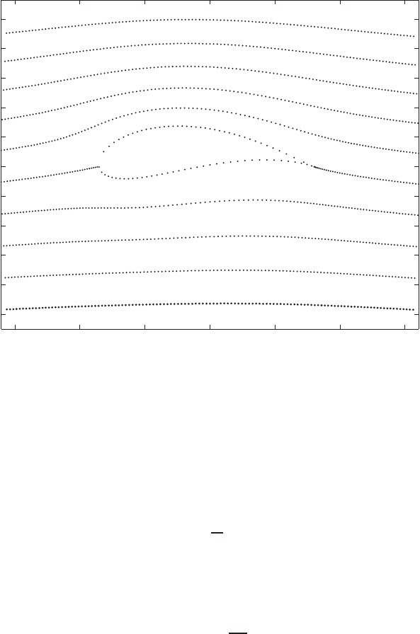
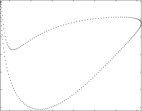
Figure 2.6.4 shows the shape of the airfoil, which is described by the stream-

line ψ = 0. The coordinates of the surface points can easily be printed out if

so desired. The plot reveals that the space between the body and the stream-

line ψ = 0.5 is narrower than that between the body and the streamline ψ =

−0.5, indicating that the speed on the upper surface is higher than that on the

lower. The corresponding pressure distributions on the upper and lower surfaces

of the airfoil are represented, respectively, by the lower and upper branches of

the curve plotted in Fig. 2.6.5. At the forward stagnation point where V = 0, the

pressure coefﬁcient takes on the maximum value of unity according to (2.6.26).

At the sharp trailing edge the speed is ﬁnite but not zero, although it is trans-

formed from the stagnation point Q in the x



-y



plane. The area enclosed by

the pressure distribution curve is proportional to the total lift of the airfoil. This

program may be used not only to generate airfoils of different shapes by vary-

ing the values assigned to b and y



, but also, with some modiﬁcations, to plot

86 INVISCID FLUID FLOWS

−3 −2 −1 0 1 2 3

−2.5

−2

−1.5

−1

−0.5

0.5

1.5

2.5

X–AXIS

Y–AXIS

FIGURE 2.6.4 Flow around a Joukowski airfoil.

ﬂow patterns obtained by mapping from various known ﬂows through arbitrary

transformations.

Problem 2.5 The transformation

z = z



(2.6.27)

maps the circle |z



|=1 into the line segment on the x axis between the points

x =−2andx = 2, and the region outside the circle into the entire x-y plane. It

is known that

w = U





−iα

iα





(2.6.28)

represents the complex potential for a uniform ﬂow of speed U past a cylinder

of unit radius centered at z



= 0. The ﬂow makes an angle α with the x



axis

at an inﬁnite distance from the cylinder. Under the transformation (2.6.27), the

complex potential (2.6.28) then becomes that for a uniform ﬂow past a ﬂat plate

at an angle of attack α. Plot the streamlines of this transformed ﬂow and the

CLASSIFICATION OF SECOND-ORDER PARTIAL DIFFERENTIAL EQUATIONS 87

−1.5 −1 −0.5

0 0.5 1 1.5

−2

−1.5

−1

−0.5

0.5

X–AXIS

CP : PRESSURE COEFFICIENT

FIGURE 2.6.5 Pressure distribution around the airfoil.

pressure distribution on the upper and lower surfaces of the plate. Note that the

velocity and therefore the pressure is unbounded at the edges of the plate.

Problem 2.6 If the Kutta condition is to be satisﬁed on the ﬂat plate described

in the previous problem, a circulation is required to move the rear stagnation point

on the circle in the x



-y



plane to the point (1,0), which maps into the trailing

edge of the plate. Plot the streamlines and pressure distribution and compare

them with those obtained for the case without a circulation.

2.7 CLASSIFICATION OF SECOND-ORDER PARTIAL

DIFFERENTIAL EQUATIONS

Consider a body moving through a compressible inviscid ﬂuid. The disturbances

originating from the body are propagating away in all directions at the speed

of sound. If the body moves at a speed much slower than the sonic speed,

these disturbances will ﬁnally reach inﬁnity in all directions, and the ﬂow pat-

tern will resemble that of an incompressible potential ﬂow past that body. In a

coordinate system attached to the body, the originally uniform oncoming ﬂow is

deformed upstream as well as downstream from it. However, if the body moves

at a supersonic speed, it overtakes the forward propagating disturbances so that

all the disturbances created by the body are left behind. The ﬂow pattern as

88 INVISCID FLUID FLOWS

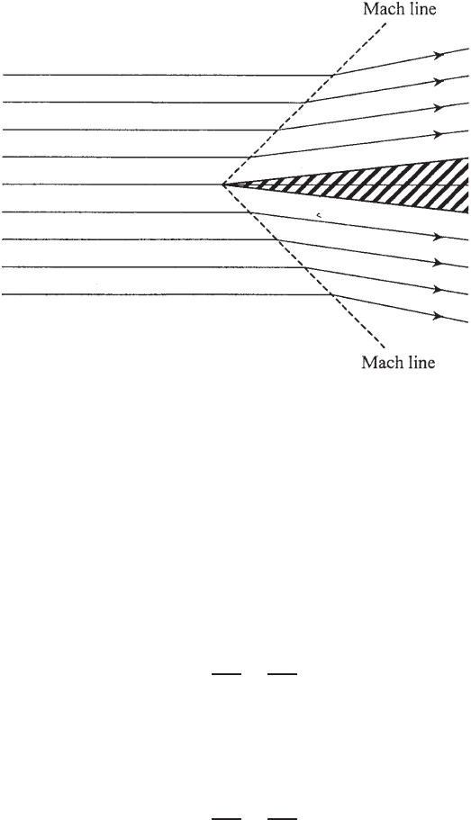
FIGURE 2.7.1 Supersonic ﬂow past a thin wedge.

seen by an observer moving with the body (e.g., a thin wedge of an inﬁnitesimal

wedge angle) is sketched in Fig. 2.7.1. The pattern is radically different from that

around a body moving subsonically in that the ﬂow upstream from the wedge is

undisturbed and remains uniform. This undisturbed region is separated from the

disturbed region along two straight lines called the Mach lines or, in mathematical

terms, the characteristics. Such lines do not exist in a subsonic ﬂow.

In fact, the governing equations for these two ﬂows are of different forms.

About a thin body that produces only weak disturbances, the governing equation

for a two-dimensional subsonic ﬂow is (Kuethe and Chow, 1998, Section 11.3)

(1 − M

)

∂

∂x

∂

∂y

= 0 (2.7.1)

in which φ is the velocity potential and M , the Mach number, is the ratio of ﬂow

speed to the speed of sound and is treated in the linearized theory as a constant.

The equation takes the following form when the ﬂow is supersonic.

−1)

∂

∂x

−

∂

∂y

= 0 (2.7.2)

Notice that in (2.7.1) the two coefﬁcients have the same sign, whereas in (2.7.2)

their signs are opposite. These two partial differential equations are said to be of

two different types.

The type of an equation is determined by examining the existence of charac-

teristics along which two different solutions to the same equation may be patched

CLASSIFICATION OF SECOND-ORDER PARTIAL DIFFERENTIAL EQUATIONS 89

(as demonstrated in Fig. 2.7.1). For a general discussion let us assume that the

velocity potential of a two-dimensional ﬂow is governed by a representative

equation

Aφ

+2Bφ

+C φ

= D (2.7.3)

in which A, B, C ,andD may be functions of x, y, φ, φ

,andφ

.Herethe

subscripts are used to denote partial derivatives, so that φ

represents ∂φ/∂x, φ

represents ∂

φ/∂x∂y, and so forth. If the velocity components φ

and φ

are

both continuous functions of x and y, their changes when going from (x, y) to a

neighboring point (x + dx, y + dy) are, respectively,

dx ·φ

+dy ·φ

+0 ·φ

= dφ

(2.7.4)

0 · φ

+dx · φ

+dy · φ

= dφ

(2.7.5)

Equations (2.7.3) to (2.7.5) may be solved simultaneously for the three second-

order derivatives of φ. For instance, by applying Cramer’s rule, we ﬁnd

ADC

dx dφ

0 dφ

A 2BC

dx dy 0

0 dx dy

(2.7.6)

However, if dx and dy are the components of a displacement along a Mach line

(i.e., a characteristic), the derivatives of velocity components in the direction of

that line may be discontinuous because along it two different solutions may be

patched. Accordingly, along a characteristic, the second-order derivatives of φ

are indeterminate. Setting the denominator of (2.7.6) equal to zero gives





−2B

+C = 0 (2.7.7)

where dy/dx is the slope of a characteristic. Its expression is obtained by solving

the preceding equation:





char

B ±

√

−AC

(2.7.8)

Similarly, by setting the numerator of (2.7.6) equal to zero, the slope of a char-

acteristic is determined in the hodograph plane using velocity components as the

coordinates.

There are three possible results for the slope of a characteristic in the physical

plane, depending on the magnitude of the expression under the radical of (2.7.8).

They are stated separately as follows.

If B

−AC > 0, there exist two characteristics at a point whose slopes are

represented by the two real values computed from the right-hand side of (2.7.8).

The partial differential equation is then classiﬁed as being of hyperbolic type.

The equations governing steady or unsteady wave motions usually belong to

90 INVISCID FLUID FLOWS

this category. One example is (2.7.2), the equation describing perturbations in a

supersonic ﬂow, in which A = M

−1, B = 0, and C =−1, so that B

−AC =

−1 > 0. The slopes of the two characteristics are ±1



√

−1 according to

(2.7.8), which are exactly the slopes of Mach lines in a supersonic ﬂow (Kuethe

and Chow, 1998, p. 273).

If B

−AC > 0, the right-hand side of (2.7.8) becomes complex. The existence

of characteristics is impossible, and the corresponding partial differential equation

is classiﬁed as being of elliptic type. Examples are the Laplace and Poisson

equations introduced in Section 2.1 for incompressible potential ﬂows, and the

governing subsonic equation (2.7.1). In the latter case A = 1 −M

, B = 0, and

C = 1 and, therefore, B

−4AC =−(1 −M

)<0.

Finally, if B

−4AC = 0, there is only one real value for the slope, and such

a partial differential equation is called of parabolic type. The following example

is the equation governing the unsteady thermal conduction in a one-dimensional

conductor:

∂T

∂t

= k

∂

∂x

(2.7.9)

where T denotes temperature, x and t represent, respectively, spatial coordinate

and time, and k is the thermal diffusivity of the conducting medium. A com-

parison between (2.7.9) and the standard form (2.7.3) gives A = k, B = C = 0,

so that B

−AC = 0. It will be shown in the next chapter that the equation

describing diffusion of vorticity in a viscous ﬂuid also belongs to this class.

These three types of partial differential equations may be solved using different

numerical techniques, which will be introduced in this and the following chapters.

2.8 NUMERICAL METHODS FOR SOLVING ELLIPTIC PARTIAL

DIFFERENTIAL EQUATIONS

Suppose that the Poisson equation

∂

∂x

∂

∂y

= q(x, y) (2.8.1)

which is an elliptic partial differential equation, is to be solved in a rectangular

region subject to the condition that the values of f are prescribed on the boundary

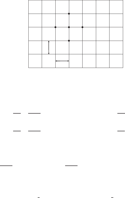
of that domain. To introduce a commonly used numerical technique, we refer to

the rectangular grid system shown in Fig. 2.8.1. We use the notation (i, j ) to

indicate the intersecting point of the vertical grid line passing through x

and

the horizontal grid line through y

. Our ﬁrst step is to approximate the partial

differential equation (2.8.1) by a ﬁnite difference equation at the representative

interior point (i, j).

Let f

i, j

and q

i, j

represent f (x

, y

) and q(x

, y

), respectively. Applying the

central-difference formula (2.2.9) for computing second-order derivatives and

NUMERICAL METHODS FOR SOLVING ELLIPTIC PARTIAL DIFFERENTIAL EQUATIONS 91

Δy

Δx

(i + 1, j )(i, j )(i − 1, j )

(i, j + 1)

(i, j − 1)

FIGURE 2.8.1 Rectangular domain.

referring to the ﬁve neighboring points as shown in Fig. 2.8.1, we have

∂

∂x

(x)

i+1, j

−2f

i, j

i−1, j

) −O



(x)



∂

∂x



i, j



∂

∂y

(y)

i, j +1

−2f

i, j

i, j −1

) − O



(y)



∂

∂y



i, j



The differential equation (2.8.1) may then be replaced by the ﬁnite-difference

form

(x)

i+1, j

−2f

i, j

i−1, j

) +

(y)

i, j +1

−2f

i, j

i, j −1

) = q

i, j

(2.8.2)

with a truncation error of the order of (x)

+(y)

For a square grid we let x = y = h, so that the preceding equation becomes

i, j

i−1, j

i+1, j

i, j −1

i, j +1

) −

i, j

(2.8.3)

Vanishing o f q reduces (2.8.1) to the Laplace equation, and (2.8.3) states that

the value of f at an interior point is equal to the average of the values of f at

the four adjoining points. This statement is called the mean value theorem for

harmonic functions that satisfy the Laplace equation.

When (2.8.2) or (2.8.3) is applied at all interior points bounded within the

domain of Fig. 2.8.1, we obtain (m −2)(n − 2) algebraic equations that automat-

ically include the boundary conditions. Solving these equations simultaneously,

we can, theoretically, ﬁnd the unknown values of f at the interior grid points.