Bednorz W. (ed.) Advances in Greedy Algorithms
Подождите немного. Документ загружается.


A Multilevel Greedy Algorithm for the Satisfiability Problem
41
and error. Typically, they start with an initial assignment of the variables, either randomly or
heuristically generated. Satisfiability can be formulated as an optimization problem in which
the goal is to minimize the number of unsatisfied clauses. Thus, the optimum is obtained
when the value of the objective function equals zero, which means that all clauses are
satisfied. During each iteration, a new solution is selected from the neighborhood of the
current one by performing a move. Choosing a good neighborhood and a search method are
usually guided by intuition, because very little theory is available as a guide. Most SLS
algorithms use a 1-flip neighborhood relation for which two truth value assignments are
neighbors if they differ in the truth value of one variable. If the new solution provides a
better value in light of the objective function, the new solution replaces the current one. The
search terminates if no better neighbor solution can be found.
One of the most popular local search methods for solving SAT is GSAT [9]. The GSAT
algorithm operates by changing a complete assignment of variables into one in which the
maximum possible number of clauses are satisfied by changing the value of a single
variable. An extension of GSAT referred as random-walk [10] has been realized with the
purpose of escaping from local optima. In a random walk step, an unsatisfied clause is
randomly selected. Then, one of the variables appearing in that clause is flipped, thus
effectively forcing the selected clause to become satisfied. The main idea is to decide at each
search step whether to perform a standard GSAT or a random-walk strategy with a
probability called the walk probability. Another widely used variant of GSAT is the
WalkSAT algorithm originally introduced in [12]. It first picks randomly an unsatisfied
clause and then in a second step, one of the variables with the lowest break count appearing
in the selected clause is randomly selected. The break count of a variable is defined as the
number of clauses that would be unsatisfied by flipping the chosen variable. If there exists a
variable with break count equals to zero, this variable is flipped, otherwise the variable with
minimal break count is selected with a certain probability (noise probability). The choice of
unsatisfied clauses combined with the randomness in the selection of variables enable
WalkSAT to avoid local minima and to better explore the search space.
Recently, new algorithms [12] [13] [14] [15] [16] have emerged using history-based variable
selection strategy in order to avoid flipping the same variable. Apart from GSAT and its
variants, several clause weighting based SLS algorithms [17] [18] have been proposed to
solve SAT problems. The key idea is associate the clauses of the given CNF formula with
weights. Although these clause weighting SLS algorithms differ in the manner how clause
weights should be updated (probabilistic or deterministic) they all choose to increase the
weights of all the unsatisfied clauses as soon as a local minimum is encountered. Clause
weighting acts as a diversification mechanism rather than a way of escaping local minima.
Finally, many other SLS algorithms have been applied to SAT. These include techniques
such as Simulated Annealing [19], Evolutionary Algorithms [20], and Greedy Randomized
Adaptive Search Procedures [21].
3. The GSAT greedy algorithm
This section is devoted to explaining the GSAT greedy algorithm and one of its variants
before embedding it into the multilevel paradigm. Basically, the GSAT algorithm begins
with a randomly generated assignment of the variables, and then uses the steepest descent
Advances in Greedy Algorithms
42
heuristic to find the new truth value assignment which best decreases the number of
unsatisfied clauses. After a fixed number of moves, the search is restarted from a new
random assignment. The search continues until a solution is found or a fixed number of
restart is performed. As with any combinatorial optimization , local minima or plateaus (i.e.,
a set of neighboring states each with an equal number of unsatisfied clauses) in the search
space are problematic in the application of greedy algorithms. A local minimum is defined
as a state whose local neighborhood does not include a state that is strictly better. The
introduction of an element of randomness (e.g., noise) into a local search methods is a
common practice to increase the success of GSAT and improve its effectiveness through
diversification [2].
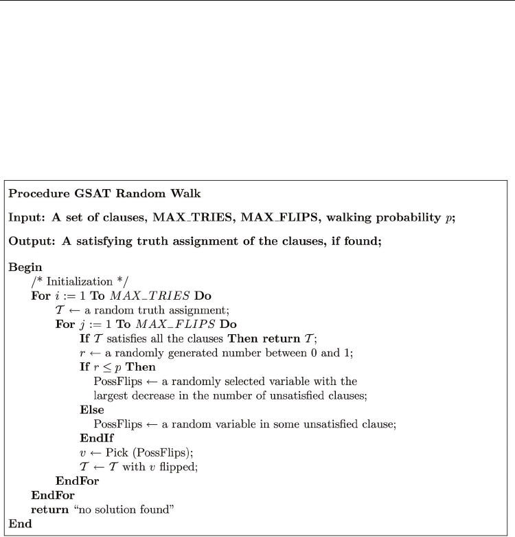
Fig. 1. The GSAT Random Walk Algorithm.
The algorithm of GSAT Random Walk, which is shown in Figure 1, starts with a randomly
chosen assignment. Thereafter two possible criteria are used in order to select the variable to
be flipped. The first criterion uses the notion of a “noise” or walk-step probability to
randomly select a currently unsatisfied clause and flip one of the variables appearing in it
also in a random manner. At each walk-step, at least one unsatisfied clause becomes
satisfied. The other criterion uses a greedy search to choose a random variable from the set
PossFlips. Each variable in this set, when flipped, can achieve the largest decrease (or the
least increase) in the total number of unsatisfied clauses. The walk-step strategy may lead to
an increase in the total number of unsatisfied clauses even if improving flips would have
been possible. In consequence, the chances of escaping from local minima of the objective
function are better compared with the basic GSAT [11].
A Multilevel Greedy Algorithm for the Satisfiability Problem
43
4. The multilevel paradigm
The multilevel paradigm is a simple technique which at its core applies recursive coarsening
to produce smaller and smaller problems that are easier to solve than the original one.
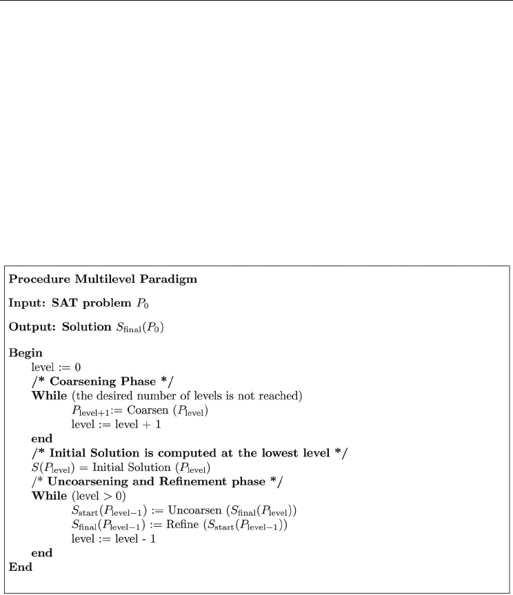
Figure 2 shows the generic multilevel paradigm in pseudo-code. The multilevel paradigm
consists of three phases: coarsening, initial solution, and multilevel refinement. During the
coarsening phase, a series of smaller problems is constructed by matching pairs of vertices
of the input original problem in order to form clusters, which define a related coarser
problem. The coarsening procedure recursively iterates until a sufficiently small problem is
obtained. Computation of an initial solution is performed on the coarsest level (the smallest
problem). Finally, the initial solution is projected backward level by level. Each of the finer
levels receives the preceding solution as its initial assignment and tries to refine it by some
local search algorithm. A common feature that characterizes multilevel algorithms is that
any solution in any of the coarsened problems is a legitimate solution to the original
problem. This is always true as long as the coarsening is achieved in a way that each of the
coarsened problems retains the original problem’s global structure.
Fig. 2. The Multilevel Generic Algorithm.
The key success behind the efficiency of the multilevel techniques is the use of the multilevel
paradigm, which offers two main advantages enabling local search techniques to become
much more powerful in the multilevel context. First, by allowing local search schemes to
view a cluster of vertices as a single entity, the search becomes restricted to only those
configurations in the solution space in which the vertices grouped within a cluster are
assigned the same label. During the refinement phase a local refinement scheme applies a
local transformation within the neighborhood (i.e., the set of solutions that can be reached

Advances in Greedy Algorithms
44
from the current one) of the current solution to generate a new one. As the size of the
clusters varies from one level to another, the size of the neighborhood becomes adaptive and
allows the possibility of exploring different regions in the search space. Second, the ability of
a refinement algorithm to manipulate clusters of vertices provides the search with an
efficient mechanism to escape from local minima.
Multilevel techniques were first introduced when dealing with the graph partitioning
problem (GPP) [1] [5] [6] [7] [8] [22] and have proved to be effective in producing high
quality solutions at lower cost than single level techniques. The traveling salesman problem
(TSP) was the second combinatorial optimization problem to which the multilevel paradigm
was applied and has clearly shown a clear improvement in the asymptotic convergence of
the solution quality. Finally, when the multilevel paradigm was applied to the graph
coloring problem, the results do not seem to be in line with the general trend observed in
GPP and TSP as its ability to enhance the convergence behaviour of the local search
algorithms was rather restricted to some problem classes.
5. A multilevel framework for SAT
• Coarsening: The original problem P
0
is reduced into a sequence of smaller problems P
0
,
P
2
, . . . , P
m
. It will require at least O(log n/n’) steps to coarsen an original problem with n
variables down to n’ variables. Let
V
v
i
denote the set of variables of P
i
that are combined
to form a single variable v in the coarser problem P
i+1
. We will refer to v as a
multivariable. Starting from the original problem P
0
, the first coarser problem P
1
is
constructed by matching pairs of variables of P
0
into multivariables. The variables in P
0
are visited in a random order. If a variable has not been matched yet, then we randomly
select another unmatched variable, and a multivariable consisting of these two variables
is created. Unmatchable variables are simply copied to the coarser level. The new
multivariables are used to define a new and smaller problem. This coarsening process is
recursively carried out until the size of the problem reaches some desired threshold.
• Initial solution: An initial assignment
A
m
of P
m
is easily computed using a random
assignment algorithm, which works by randomly assigning to each multivariable of the
coarsest problem P
m
the value of true or false.
• Projection: Having optimized the assignment A
k+1
for P
k+1
, the assignment must be
projected back to its parent P
k
. Since each multivariable of P
k+1
contains a distinct subset
of multivariables of P
k
, obtaining A
k
from A
k+1
is done by simply assigning the set of
variables
V
k
v
the same value as v ∈ P
k+1
(i.e., A
k
[u] = A
k+1
[v], ∀u ∈V
k
v
).
• Refinement: At each level, the assignment from the previous coarser level is projected
back to give an initial assignment and further refined. Although
A
k+1
is a local minimum
of P
k+1
, the projected assignment A
k
may not be at a local optimum with respect to P
k
.
Since P
k
is finer, it may still be possible to improve the projected assignment using a
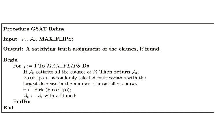
version of GSAT adapted to the multilevel paradigm. The idea of GSAT refinement as
shown in Figure 3 is to use the projected assignment of P
k+1
onto P
k
as the initial
assignment of GSAT. Since the projected assignment is already a good one, GSAT will
hopefully converge quickly to a better assignment. During each level, GSAT is allowed
to perform MAXFLIPS iterations before moving to a finer level. If a solution is not
A Multilevel Greedy Algorithm for the Satisfiability Problem
45
found at the finest level, a new round of coarsening, random initial assignment, and
refinement is performed.
Fig. 3. The GSAT Refinement Algorithm.
6. Experimental results
6.1 Benchmark instances
To illustrate the potential gains offered by the multilevel greedy algorithm, we selected a
benchmark suite from different domains including benchmark instances of SAT competition
Beijing held in 1996. These instances are by no means intended to be exhaustive but rather
as an indication of typical performance behavior. All these benchmark instances are known
to be hard and difficult to solve and are available from the SATLIB website
(http://www.informatik.tudarmstadt. de/AI/SATLIB). All the benchmark instances used
in this section are satisfiable and have been used widely in the literature in order to give an
overall picture of the performance of different algorithms. Due to the randomization of the
algorithm, the time required for solving a problem instance varies between different runs.
Therefore, for each problem instance, we run GSAT and MLVGSAT both 100 times with a
max-time cutoff parameter set to 300 seconds. All the plots are given in logarithmic scale
showing the evolution of the solution quality based on averaged results over the 100 runs.
6.1.1 Random-3-SAT
Uniform Random-3-SAT is a family of SAT problems obtained by randomly generating 3-
CNF formula in the following way: For an instance with n variables and k clauses, each of
the k clauses is constructed from 3 literals which are randomly drawn from the 2n possible
literals (the n variables and their negations), such that each possible literal is selected with
the same probability of 1/2n. Clauses are not accepted for the construction of the problem
instance if they contain multiple copies of the same literal or if they are tautological (i.e.,
they contain a variable and its negation as a literal).
6.1.2 SAT-encoded graph coloring problems
The graph coloring problem (GCP) is a well-known combinatorial problem from graph
theory: Given a graph G = (
V, E), where V = v
1
, v
2
, . . . , v
n
is the set of vertices and E the set of

Advances in Greedy Algorithms
46
edges connecting the vertices, the goal is to find a coloring
C : V → N, such that two vertices
connected by an edge always have different colors. There are two variants of this problem:
In the optimization variant, the goal is to find a coloring with a minimal number of colors,
whereas in the decision variant, the question is to decide whether for a particular number of
colours, a coloring of the given graph exists. In the context of SAT-encoded graph coloring
problems, we focus on the decision variant.
6.1.3 SAT-encoded logistics problems
In the logistics planning domain, packages have to be moved between different locations in
different cities. Within cities, packages are carried by trucks while between cities they are
transported by planes. Both trucks and airplanes are of limited capacity. The problem
involves 3 operators (load, unload, move) and two state predicates (in, at). The initial and
goal state specify locations for all packages, trucks, and planes; the plans allow multiple
actions to be executed simultaneously, as long as no conflicts arise from their preconditions
and effects. The question in the decision variant is to decide whether a plan of a given length
exists. SAT-based approaches to logistics planning typically focus on the decision variant.
6.1.4 SAT-encoded block world planning problems
The Blocks World is a very well-known problem domain in artificial intelligence research.
The general scenario in Blocks World Planning comprises a number of blocks and a table.
The blocks can be piled onto each other, where the down-most block of a pile is always on
the table. There is only one operator which moves the top block of a pile to the top of
another pile or onto the table. Given an initial and a goal configuration of blocks, the
problem is to find a sequence of operators which, when applied to the initial configuration,
leads to the goal situation. Such a sequence is called a (linear) plan. Blocks can only be
moved when they are clear, i.e., no other block is piled on top of them, and they can be only
moved on top of blocks which are clear or onto the table. If these conditions are satisfied, the
move operator always succeeds. SAT-based approaches to Blocks World Planning typically
focus on the decision variant where the question is to decide whether a plan of a given
length exists.
6.1.5 SAT-encoded quasigroup problems
A quasigroup is an ordered pair (
Q, ·), where Q is a set and · is a binary operation on Q such
that the equations a · x = b and y · a = b are uniquely solvable for every pair of elements a, b
in
Q. The cardinality of the set Q is called the order of the quasigroup. Let N be the order of
the quasigroup
Q then the multiplication table Q is a table N ×N such that the cell at the
coordinate (x, y) contains the result of the operation x · y. The multiplication of the
quasigroup must satisfy a condition that there are no repeated result in each row or column.
Thus, the multiplication table defines a Latin square. A complete Latin square is a table that
is filled completely. The problem of finding a complete Latin square can be stated as a
satisfiability problem.
6.2 Experimental results
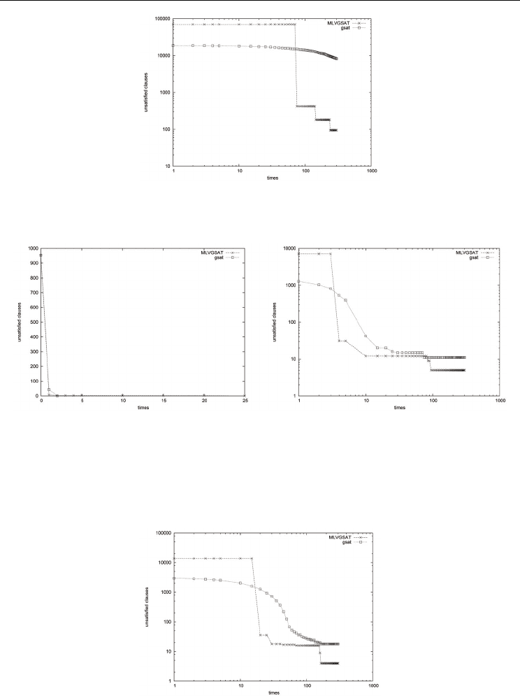
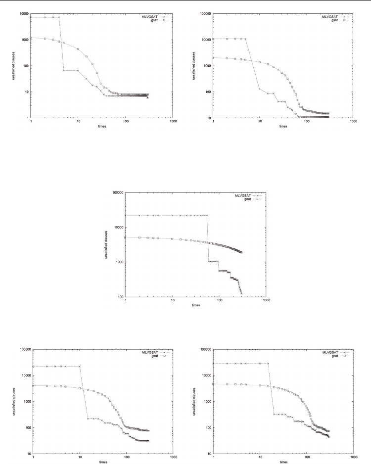
Figures 4-15 show individual results which appear to follow the same pattern within each
application domain. Overall, at least for the instances tested here, we observe that the search

A Multilevel Greedy Algorithm for the Satisfiability Problem
47
pattern happens in two phases. In the first phase, both MLVGSAT and GSAT behave as a
hill-climbing method. This phase is short and a large number of the clauses are satisfied. The
best assignment climbs rapidly at first, and then flattens off as we mount the plateau,
marking the start of the second phase. The plateau spans a region in the search space where
flips typically leave the best assignment unchanged. The long plateaus become even more
pronounced as the number of flips increases, and occurs more specifically in trying to satisfy
the last few remaining clauses. The transition between two plateaus corresponds to a change
to the region where a small number of flips gradually improve the score of the current
solution ending with an improvement of the best assignment. The plateau is rather of short
length with MLVGSAT compared with that of GSAT. For MLVGSAT the projected solution
from one level to its finer predecessor offers an elegant mechanism to reduce the length of
the plateau as it consists of more degrees of freedom that can be used for further improving
the best solution. The plots show a time overhead for MLVGSAT specially for large
problems due mainly to data structures settings at each level. We feel that this initial
overhead, which is a common feature in multilevel implementations is more susceptible to
further improvements, and will be considerably minimized by a more efficient
implementation. Comparing GSAT and MLVGSAT for small problems (up to 1500 clauses)
and as can be seen from the left sides of Figures 6,8, both algorithms seem to be reaching the
optimal quality solutions. It is not immediately clear which of the two algorithms converges
more rapidly. This is probably very dependent on the choice of the instances in the test
suite. For example the run time required by MLVGSAT for solving instance flat100-239 is
more than 12 times higher than the mean run-time of GSAT (25sec vs 2sec). The situation is
reversed when solving the instance block-medium (20sec vs 70sec). The difference in
convergence behavior of the two algorithms becomes more distinctive as the size of the
problem increases. All the plots show a clear dominance of MLGSAT over GSAT
throughout the whole run. MLVGSAT shows a better asymptotic convergence (to around
0.008%−0.1%) in excess of the optimal solution as compared with GSAT which only reach
around (0.01%- 11%). The performance of MLVGSAT surpasses that of GSAT although few
of the curves overlay each other closely, MLVGSAT has marginally better asymptotic
convergence.
The quality of the solution may vary significantly from run to run on the same problem
instance due to random initial solutions and subsequent randomized decisions. We choose
the Wilcoxon Rank test in order to test the level of statistical confidence in differences
between the mean percentage excess deviation from the solution of the two algorithms. The
test requires that the absolute values of the differences between the mean percentage excess
deviation from the solution of the two algorithms are sorted from smallest to largest and
these differences are ranked according to the absolute magnitude. The sum of the ranks is
then formed for the negative and positive differences separately. As the size of the trials
increases, the rank sum statistic becomes normal. If the null hypothesis is true, the sum of
ranks of the positive differences should be about the same as the sum of the ranks of the
negative differences. Using two-tailed P value, significance performance difference is
granted if the Wilcoxon test is significant for P < 0.05.
Looking at Table 1, we observe that the difference in the mean excess deviation from the
solution is significant for large problems and remains insignificant for small problems.
Advances in Greedy Algorithms
48
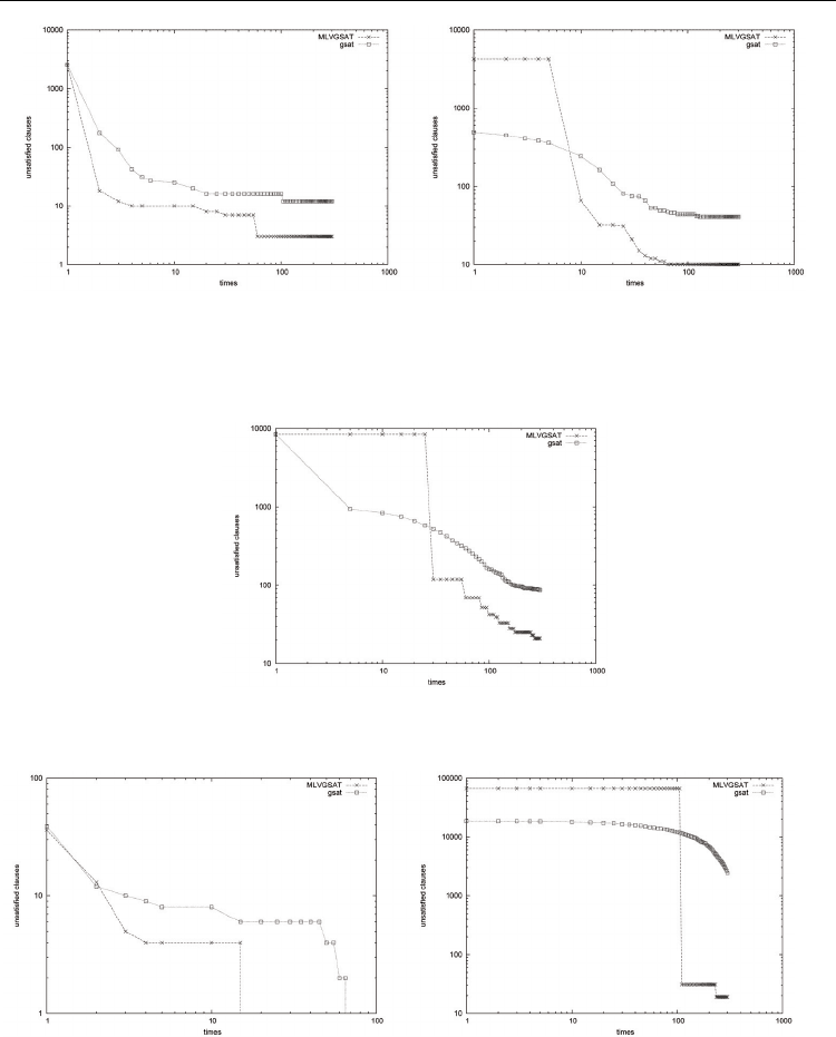
Fig. 4. Log-Log plot:Random:(Left ) Evolution of the best solution on a 600 variable problem
with 2550 clauses (f600.cnf). Along the horizontal axis we give the time in seconds , and
along the vertical axis the number of unsatisfied clauses. (Right) Evolution of the best
solution on a 1000 variable problem with 4250 clauses. (f1000.cnf).Horizontal axis gives the
time in seconds, and the vertical axis shows the number of unsatisfied clauses.
Fig. 5. Log-Log plot: Random:Evolution of the best solution on a 2000 variable problem with
8500 clauses (f2000.cnf). Along the horizontal axis we give the time in seconds , and along
the vertical axis the number of unsatisfied clauses.
Fig. 6. Log-Log plot: SAT-encoded graph coloring:(Left ) Evolution of the best solution on a
300 variable problem with 1117 clauses (flat100.cnf). Along the horizontal axis we give the
time in seconds, and along the vertical axis the number of unsatisfied clauses. (Right)
Evolution of the best solution on a 2125 variable problem with 66272 clauses (g125-17.cnf).
Horizontal axis gives the time in seconds, and the vertical axis shows the number of
unsatisfied clauses.
A Multilevel Greedy Algorithm for the Satisfiability Problem
49
Fig. 7. Log-Log plot: SAT-encoded graph coloring:Evolution of the best solution on a 2250
variable problem with 70163 clauses (g125-18.cnf). Along the horizontal axis we give the
time in seconds , and along the vertical axis the number of unsatisfied clauses.
Fig. 8. SAT-encoded block world:(Left ) Evolution of the best solution on a 116 variable
problem with 953 clauses (medium.cnf). Along the horizontal axis we give the time in
seconds , and along the vertical axis the number of unsatisfied clauses. Log-Log plot (Right)
Evolution of the best solution on a 459 variable problem with 7054 clauses (huge.cnf).
Horizontal axis gives the time in seconds, and the vertical axis shows the number of
unsatisfied clauses.
Fig. 9. Log-Log plot: SAT-encoded block world:Evolution of the best solution on a 1087
variable problem with 13772 clauses (bw-largeb.cnf). Along the horizontal axis we give the
time in seconds, and along the vertical axis the number of unsatisfied clauses.
Advances in Greedy Algorithms
50
Fig. 10. Log-Log plot: SAT-encoded Logistics:(Left) Evolution of the best solution on a 843
variable problem with 7301 clauses (logisticsb.cnf). Along the horizontal axis is the time in
seconds , and along the vertical axis the number of unsatisfied clauses. (Right) Evolution of
the best solution on a 1141 variable problem with 10719 clauses (logisticsc.cnf). Horizontal
axis gives the time in seconds, and the vertical axis shows the number of unsatisfied clauses.
Fig. 11. Log-Log plot:SAT-encoded logistics:Evolution of the best solution on a 4713 variable
problem with 21991 clauses (logisticsd.cnf). Along the horizontal axis we give the time in
seconds, and along the vertical axis the number of unsatisfied clauses.
Fig. 12. Log-Log plot:SAT-encoded quasigroup:(Left) Evolution of the best solution on a 129
variable problem with 21844 clauses (qg6-9.cnf). Along the horizontal axis we give the time
in seconds , and along the vertical axis the number of unsatisfied clauses.(Right) Evolution
of the best solution on a 729 variable problem with 28540 clauses (qg5.cnf). Horizontal axis
gives the time in seconds, and the vertical axis shows the number of unsatisfied clauses.
