Bednorz W. (ed.) Advances in Greedy Algorithms

Подождите немного. Документ загружается.

A Greedy Algorithm with Forward-Looking Strategy

At each iteration, a set of CCOAs for each of the unpacked rectangles is generated under

current configuration C. Then the CCOAs for all the unpacked rectangles outside the

container are gathered as a list L. A

calculates the degree of each CCOA in L and selects the

CCOA (i, x, y,

) with the highest degree

, and place rectangle i at (x, y) with orientation

After placing rectangle i, the list L is modified as follows:

1. Remove all the CCOAs involving rectangle i;

2. Remove all infeasible CCOAs. A CCOA becomes infeasible because the involved

rectangle would overlap rectangle i if it was placed;

3. Re-calculate the degree

of the remaining CCOAs;

4. If a rectangle outside the container can be placed inside the container without overlap

so that it touches rectangle i and a rectangle inside the container or the side of the

container, create a new CCOA and put it into L, and compute the degree

of the new

CCOA.

If none of the rectangles outside the container can be packed into the container without

overlap (L is empty) at certain iteration, A

stops with failure (returns a failure

configuration). If all rectangles are packed in the container without overlap, A

stops with

success (returns a successful configuration).

It should be pointed out that if there are several CCOAs with the same highest degree, we

will select one that packs the corresponding rectangle closest to the bottom left corner of the

container.

is a fast algorithm. However, given a configuration, A

only considers the relation

between the rectangles already inside the container and the rectangle to be packed. It

doesn’t examine the relation between the rectangles outside the container. In order to more

globally evaluate the benefit of a CCOA and to overcome the limit of A

, we compute the

benefit of a CCOA using A

itself in the procedure BenefitA

to obtain our main packing

algorithm called A

4.4 The greedy algorithm with forward-looking strategy: A

Based on current configuration C, CCOAs for all unpacked rectangles are gathered as a list

L. For each CCOA (i, x, y,

) in L, the procedure BenefitA

is designed to evaluate its benefit

more globally.

Procedure BenefitA

(i, x, y,

, C, L)

Begin

let C’and L’be copies of C and L;

modify C’by placing rectangle i at (x, y) with orientation

, and modify L’;

C’= A

(C’,L’);

if (C’is a successful configuration)

Return C’;

else

Return density (C’);

end if-else

End.

Given a copy C’ of the current configuration C and a CCOA (i, x, y,

) in L, BenefitA

begins

by packing rectangle i in the container at (x, y) with orientation

and call A

to reach a final

configuration. If A

stops with success then BenefitA

returns a successful configuration,

Advances in Greedy Algorithms

otherwise BenefitA

returns the density (the ratio of the total area of the rectangles inside the

container to the area of the container) of a failure configuration as the benefit of the CCOA

(i, x, y,

). In this manner, BenefitA

evaluates all existing CCOAs in L.

Now, using the procedure BenefitA

, the benefit of a CCOA is measured by the density of a

failure configuration. The main algorithm A

is presented as follow:

Procedure A

( )

Begin

generate the initial configuration C;

generate the initial CCOA list L;

while (L is not empty)

maximum benefit

←

for each CCOA (i, x, y,

) in L

d= BenefitA

(i, x, y,

, C, L);

if (d is a successful configuration)

stop with success;

else

update the maximum benefit with d;

end if-else;

end for;

select the CCOA (

i ,

) with the maximum benefit;

modify C by placing rectangle

i at (

) with orientation

;

modify L according to the new configuration C;

end while;

stop with failure

End.

Similarly, A

selects the CCOA with the maximum benefit and packs the corresponding

rectangle into the container by this CCOA at each iteration. If there are several CCOAs with

the maximum benefit, we select one that packs the corresponding rectangle closest to the

bottom left corner of the container.

4.5 Computational complexity

We analysis the complexity of A

in the worst case, that is, when it cannot find successful

configuration, and discuss the real computational cost to find a successful configuration.

is clearly polynomial. Since every pair of rectangles or sides in the container can give a

possible CCOA for a rectangle outside the container, the length of L is bounded by

O(m

(n−m)), if m rectangles are already placed in the container. For each CCOA in L, d

min

calculated using the d

min

in the last iteration in O(1) time. The creation of new CCOAs and

the calculus of their degree is also bounded by O(m

(n−m)) since there are at most

O(m(n−m)) new CCOAs (a rectangle might form a corner position with each rectangle in the

container and each side of the container). So the time complexity of A

is bounded by O(n

uses a powerful search strategy in which the consequence of each CCOA is evaluated by

applying BenefitA

in full, which allows us to examine the relation between all rectangles

(inside and outside the container). Note that the benefit of a CCOA is measured by the

A Greedy Algorithm with Forward-Looking Strategy

density of a final configuration, which means that we should apply BenefitA

though to the

end each time. At every iteration of A

, BenefitA

uses a O(n

) procedure to evaluate all

O(m

(n−m)) CCOAs, therefore, the complexity of A

is bounded by O(n

It should be pointed out that the above upper bounds of the time complexity of A

and A

are just rough estimations, because most corner positions are infeasible to place any

rectangle outside the container, and the real number of CCOAs in a configuration is thus

much smaller than the theoretical upper bound O(m

(n−m)).

The real computational cost of A

and A

to find a successful configuration is much smaller

than the above upper bound. When a successful configuration is found, BenefitA

does not

continue to try other CCOAs, nor A

to exhaust the search space. In fact, every call to A

BenefitA

may lead to a successful configuration and then stops the execution at once. Then,

the real computational cost of A

essentially depends on the real number of CCOAs in a

configuration and the distribution of successful configurations. If the container height is not

close to the optimal one, there exists many successful configurations, and A

can quickly

find such one. However, if the container height is very close to the optimal one, few

successful configurations exist in the search space, and then A

may need to spend more

time to find a successful configuration in this case.

4.6 Computational results

The set of tests is done using the Hopper and Turton instances [6]. There are 21 different sized

test instances ranging from 16 to 197 items, and the optimal packing solutions of these test

instances are all known (see Table 1). We implemented A

in C on a 2.4 GHz PC with 512 MB

memory. As shown in Table 1, A

generates optimal solutions for 8 of the 21 instances; for the

remaining 13 instances, the optimum is missed in each case by a single length unit.

To evaluate the performance of the algorithm, we compare A

with two best meta-heuristic

(SA+BLF) in [6], HR [7], LFFT [8] and SPGAL [9]. The quality of a solution is measured by

the percentage gap, i.e., the relative distance of the solution lU to the optimum length lOpt.

The gap is computed as (lU − lOpt)/lOpt. The indicated gaps for the seven classes are

averaged over the respective three instances. As shown in Table 2, the gaps of A

ranges

form 0.0% to 1.64% with the average gap 0.72, whereas the average gap of the two meta-

heuristics and HR are 4.6%, 4.0% and 3.97%, respectively. Obviously, A

considerably

outperforms these algorithms in terms of packing density. Compared with two other

methods, the average gap of A

is lower than that of LFFT, however, the average gap of A

slightly higher than that of SPGAL.

As shown in Table 2, with the increasing of the number of rectangles, the running time of

the two meta-heuristics and LFFT increases rather fast. HR is a fast algorithm, whose time

complexity is only O(n3) [7]. Unfortunately, the running time of each instance for SPGAL is

not reported in the literature. The mean time of all test instances for SPGAL is 139 seconds,

which is acceptable in practical applications. It can be seen that A

is also a fast algorithm.

Even for the problem instances of larger size, A

can yield solutions of high density within

short running time.

It has shown from Table 2 that the running time of A

does not consistently accord with its

theoretical time complexity. For example, the average time of C3 is 1.71 seconds, while the

average time of C4 and C5 are both within 0.5 seconds. As pointed out in the time

complexity analysis, once A

finds a successful solution, the calculation of A

will terminate.

Actually, the average time complexity is much smaller than the theoretical upper bound.

Advances in Greedy Algorithms

Test instance

Class /

subclass

No. of

pieces

Object

dimensions

Optimal

height

Minimum

Height by A

% of

unpacked

area

CPU time

(s)

C11 16 20×20 20 20 0.00 0.37

C1 C12 17 20×20 20 20 0.00 0.50

C13 16 20×20 20 20 0.00 0.23

C21 25 15×40 15 15 0.00 0.59

C2 C22 25 15×40 15 15 0.00 0.44

C23 25 15×40 15 15 0.00 0.79

C31 28 30×60 30 30 0.00 3.67

C3 C32 29 30×60 30 30 0.00 1.44

C33 28 30×60 30 31 3.23 0.03

C41 49 60×60 60 61 1.64 0.22

C4 C42 49 60×60 60 61 1.64 0.13

C43 49 60×60 60 61 1.64 0.11

C51 73 90×60 90 91 1.09 0.34

C5 C52 73 90×60 90 91 1.09 0.33

C53 73 90×60 90 91 1.09 0.52

C61 97 120×80 120 121 0.83 8.73

C6 C62 97 120×80 120 121 0.83 0.73

C63 97 120×80 120 121 0.83 2.49

C71 196 240×160 240 241 0.41 51.73

C7 C72 197 240×160 240 241 0.41 37.53

C73 196 240×160 240 241 0.41 45.81

Table 1. Computational results of our algorithm for the test instances from Hopper and

Turton instances

SA+BLF

LFFT

SPGAL

Class

Gap Time Gap Time Gap Time Gap

Time

(s)

Gap Time

C1 4.0 42 8.33 0 0.0 1 1.7 − 0.00 0.37

C2 6.0 144 4.45 0 0.0 1 0.0 − 0.00 0.61

C3 5.0 240 6.67 0.03 1.0 2 2.2 − 1.07 1.71

C4 3.0 1980 2.22 0.14 2.0 15 0.0 − 1.64 0.15

C5 3.0 6900 1.85 0.69 1.0 31 0.0 − 1.09 0.40

C6 3.0 22920 2.5 2.21 1.0 92 0.3 − 0.83 3.98

C7 4.0 250800 1.8 36.07 1.0 2150 0.3 − 0.41 45.02

Average

gap (%)

4.0

3.97

0.86

0.64

0.72

Table 2. The gaps (%) and the running time (seconds) for meta-heuristics, HR, LFFT, SPGAL

and A

PC with a Pentium Pro 200MHz processor and 65MB memory [11].

Dell GX260 with a 2.4 GHz CPU [15].

PC with a Pentium 4 1.8GHz processor and 256 MB memory [14].

The machine is 2GHz Pentium [16].

2.4 GHz PC with 512 MB memory.

A Greedy Algorithm with Forward-Looking Strategy

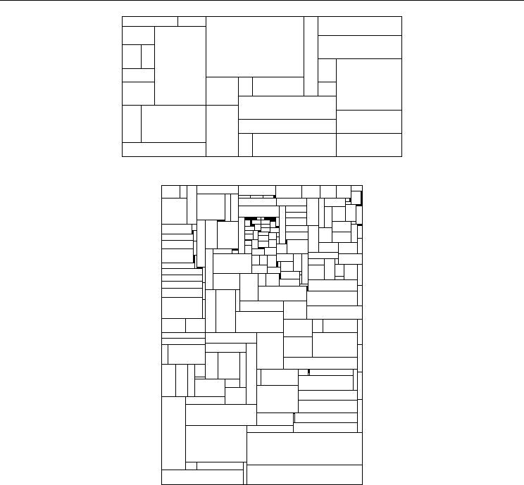
Fig. 8. Packing result of C31

Fig. 9. Packing result of C73

In addition, we give the packing results on test instances C31 and C73 for A

in Fig.8~Fig.9.

Here, the packing result of C31 is of optimal height, and the height C73 are only one length

unit higher than the optimal height

5. Conclusion

The algorithm introduced in this chapter is a growth algorithm. Growth algorithm is a

feasible approach for combinatorial optimization problems, which can be solved step by

step. After one step is taken, the original problem becomes a sub-problem. In this way, the

problem can be solved recursively. For the growth algorithm, the difficulty lies in that for a

sub-problem, there are several candidate choices for current step. Then, how to select the

most promising one is the core of growth algorithm.

By basic greedy algorithm, we use some concept to compute the fitness value of candidate

choice, then, we select one with highest value. The value or fitness is described by quantified

measure. The evaluation criterion can be local or global. In this chapter, a novel greedy

Advances in Greedy Algorithms

algorithm with forward-looking strategy is introduced, the core of which can more globally

evaluate a partial solution.

For different problems, this algorithm can be modified accordingly. This chapter gave two

new versions. One is of filtering mechanism, i.e., only part of the candidate choices with

higher local benefit will be globally evaluated. A threshold parameter is set to allow the

trade-off between solution quality and runtime effort to be controlled. The higher the

threshold parameter, the faster the search will be finished., and the lower threshold

parameter, the more high-quality solution may be expected. The other version of the greedy

algorithm is multi-level enumerations, that is, a choice is more globally evaluated.

This greedy algorithm has been successfully used to solve rectangle packing problem, circle

packing problem and job-shop problem. Similarly, it can also be applied to other

optimization problems.

6. Reference

[1] A. Dechter, R. Dechter. On the greedy solution of ordering problems. ORSA Journal on

Computing, 1989, 1: 181-189

[2] W.Q. Huang, Y Li, S Gerard, et al. A “learning from human” heuristic for solving unequal

circle packing problem. Proceedings of the First International Workshop on

Heuristics, Beijing, China, 2002, 39-45.

[3] Z. Huang, W.Q. Huang. A heuristic algorithm for job shop scheduling. Computer

Engineering & Appliances (in Chinese), 2004, 26: 25-27

[4] W.Q. Huang, Y. Li, H. Akeb, et al. Greedy algorithms for packing unequal circles into a

rectangular container. Journal of the Operational Research Society, 2005, 56: 539-548

[5] M. Chen, W.Q. Huang. A two-level search algorithm for 2D rectangular packing

problem. Computers & Industrial Engineering, 2007, 53: 123-136

[6] E. Hopper, B.Turton, An empirical investigation of meta-heuristic and heuristic

algorithms for a 2D packing problem. European J. Oper. Res, 128 (2001): 34-57

[7] D.F. Zhang, Y. Kang, A.S. Deng. A new heuristic recursive algorithm for the strip

rectangular packing problem. Computers & Operational Research. 33 (2006): 2209-

2217

[8] Y.L. Wu, C.K. Chan. On improved least flexibility first heuristics superior for packing

and stock cutting problems. Proceedings for Stochastic Algorithms: Foundations

and Applications, SAGA 2005, Moscow, 2005, 70-81

[9] A. Bortfeldt. A genetic algorithm for the two-dimensional strip packing problem with

rectangular pieces. European Journal of Operational Research. 172 (2006): 814-837

A Greedy Scheme for Designing Delay

Monitoring Systems of IP Networks

Yigal Bejerano

and Rajeev Rastogi

Bell Laboratories, Alcatel-Lucent,

Yahoo-Inc,

USA

India

1. Introduction

The demand for sophisticated tools for monitoring network utilization and performance has

been growing rapidly as Internet Service Providers (ISPs) offer their customers more services

that require quality of service (QoS) guarantees and as ISP networks become increasingly

complex. Tools for monitoring link delays and faults in an IP network are critical for numerous

important network management tasks, including providing QoS guarantees to end

applications (e.g., voice over IP), traffic engineering, ensuring service level agreement (SLA)

compliance, fault and congestion detection and performance debugging. Consequently, there

has been a recent flurry of both research and industrial activity in the area of developing novel

tools and infrastructures for measuring network parameters.

Existing network monitoring tools can be divided into two categories. Node-oriented tools

collect monitoring information from network devices (routers, switches and hosts) using

SNMP/RMON probes [1] or the Cisco NetFlow tool [2]. These are useful for collecting

statistical and billing information, and for measuring the performance of individual network

devices (e.g., link bandwidth usage). However, in addition to the need for monitoring

agents to be installed at every device, these tools cannot monitor network parameters that

involve several components, like link or end-to-end path latency. The second category

contains path-oriented tools for connectivity and latency measurement like ping,

traceroute [3], skitter [4] and tools for bandwidth measurement such as pathchar

[5], Bing [6], Cprobe [7], Nettimer [8] and pathrate [9]. As an example, skitter

sends a sequence of probe messages to a set of destinations and measures the latency of a

link as the difference in the round-trip times of the two probes to the endpoints of the link.

A benefit of path-oriented tools is that they do not require special monitoring agents to be

run at each node. However, a node with such a path-oriented monitoring tool, termed a

monitoring station, is able to measure latencies and monitor faults for only a limited set of

links in the node's routing tree, e.g., its shortest path tree (SPT). Thus, monitoring stations

need to be deployed at a few strategic points in the ISP or Enterprise IP network so as to

maximize network coverage, while minimizing hardware and software infrastructure cost,

as well as maintenance cost for the stations. Consequently, any monitoring system needs to

satisfy two basic requirements.

Advances in Greedy Algorithms

1. Coverage - The system should accurately monitor all the links and paths in the network.

2. Efficiency - The systems should minimize the overhead imposed by monitoring on the

underlying production network.

The chapter proposes an efficient two-phased approach for fully and efficiently monitoring

the latencies of links and paths using path-oriented tools. Our scheme ensures complete

coverage of measurements by selecting monitoring stations such that each network link is in

the routing trees of some monitoring station. It also reduces the monitoring overhead which

consists of two costs: the infrastructure and maintenance cost associated with the

monitoring stations, as well as the additional network traffic due to probe packets.

Minimizing the latter is especially important when information is collected frequently in

order to continuously monitor the state and evolution of the network. In the first phase, the

scheme addresses the station selection problem. This phase seeks for the locations of a minimal

set of monitoring stations that are capable to perform all the required monitoring tasks, such

as monitoring the delay of all the network links. Subsequently, in the second phase, the

scheme deals with the probe assignment problem, which computes a minimal set of probe

messages transmitted by each station for satisfying the monitoring requirements.

Although, the chapter focuses primarily on delay monitoring, the presented approach is

more generally applicable and can also be used for other management tasks. We consider

two variants of monitoring systems. A link monitoring (LM) system that guarantees that very

link is monitored by a monitoring station. Such system is useful for delay monitoring,

bottleneck links detection and fault isolation, as demonstrated in [10]. A path monitoring

(PM) system that ensures the coverage of every routing path between any pair of nodes by a

single station, which provides accurate delay monitoring.

For link monitoring we show that the problem of computing the minimum set of stations

whose routing trees (e.g, its shortest path trees), cover all network links is NP-hard.

Consequently, we map the station selection problem to the set cover problem [11], and we

use a polynomial-time greedy algorithm that yields a solution within a logarithmic factor of

the optimal one. For the probe assignment problem, we show that computing the optimal

probe set for monitoring the latency of all the network links is also NP-hard. To this

problem, we devise a polynomial-time greedy algorithm that computes a set of probes

whose cost is within an factor of 2 of the optimal solution. Then, we extend our scheme to

path monitoring. Initially, we show that even when the number of monitoring stations is

small (in our example only two monitoring stations) every pair of adjacent links along a

given routing path may be monitored by two different monitoring stations. This raises the

need for a path monitoring system in which every path is monitored by a single station. For

station selection we devise a set-cover-based greedy heuristic that computes solutions with

logarithmic approximation ratio. Then, we propose a greed algorithm for probe assignment

and leave the problem of constructing an efficient algorithm with low approximation ratio

for future work.

The chapter is organized as follows. It starts with a brief survey of related work in Section 2.

Section 3 presents the network model and a description of the network monitoring

framework is given in Section 4. Section 5 describes our link monitoring system and Section

6 extends our scheme to path monitoring. Section 7 provides simulation results that

demonstrate the efficiency of our scheme for link monitoring and Section 8 concludes the

chapter.

A Greedy Scheme for Designing Delay Monitoring Systems of IP Networks

2. Related work

The need for low-overhead network monitoring techniques has gained significant attention

in the recent years and below we provide the most relevant studies to this chapter. The

network proximity service project, SONAR [12], suggests to add a new client/server service

that enables hosts to obtain fast estimations of their distance from different locations in the

Internet. However, the problem of acquiring the latency information is not addressed. The

IDmaps [13] project produces “latency maps” of the internet using special measurement

servers called tracers that continuously probe each other to determine their distance. These

times are subsequently used to approximate the latency of arbitrary network paths.

Different methods for distributing tracers in the internet are described in [14], one of which

is to place them such that the distance of each network node to the closest tracer is

minimized. A drawback of the IDMaps approach is that latency measurements may not be

accurate. Essentially, due to the small number of paths actually monitored, it is possible for

errors to be introduced when round-trip times between tracers are used to approximate

arbitrary path latencies. In [15], Breitbart et al. propose a monitoring scheme where a single

network operations center (NOC) performs all the required measurements. In order to monitor

links not in its routing tree, the NOC uses the IP source routing option to explicitly route

probe packets along these links. The technique of using source routing for determining the

probe routes has been used by other proposals as well for both fault detection [16] and delay

monitoring [17]. Unfortunately, due to security problems, many routers frequently disable

the IP source routing option. Further, routers usually process IP options separately in their

CPU, which in addition to adversely impacting their performance, also causes packets to

suffer unknown delays. Consequently, approaches that rely on explicitly routed probe

packets for delay and fault monitoring may not be feasible in today's ISP and Enterprise

environments. Another delay monitoring approach was presented by Shavit et al. in [18].

They propose to solve a linear system of equations to compute delays for smaller path

segments from a given a set of end-to-end delay measurements for paths in the network.

The problem of station placement for delay monitoring has been addressed by several

studies. In [19], Adler et al. focus on the problem of determining the minimum cost set of

multicast trees that cover links of interest in a network, which is similar to the station

selection problem tackled in this chapter. The two-phase scheme of station placement and

probe assignment have been proposed in [10]. In this work, Bejerano and Rastogi show a

combined approach for minimizing the cost of both the monitoring stations as well as the

probe messages. Moreover, they extend their scheme for delay monitoring and fault

isolation in the presence of multiple failures. In [20] Breitbart et al. consider two variants of

the station placement problem assuming that the routing tree of the nodes are their shortest

path trees (SPTs). In the first variant, termed A-Problem, the routing trees of a node may be

any one of its SPT, while in the second variant, called E-Problem, the routing tree of a node

can be selected among all the possible SPTs for minimizing the monitoring overhead. For

both variant they have shown that the problems are NP-hard and they provided

approximation algorithms. In [21] Nguyen and Thiran developed a technique for locating

multiple failures in IP networks using active measurement. They also proposed a two-

phased approach, but unlike the work in [10], they optimize first the probe selection and

only then they compute the location of a minimal set of monitoring stations that can

generate these probes. Moreover, by using techniques from a max-plus algebra theory, they

show that the optimal set of probes can be determined in polynomial time. In [22], Suh et al.

Advances in Greedy Algorithms

propose a scheme for cost-effective placement of monitoring stations for passive monitoring

of IP flows and controlling their sampling rate. Recently, Cantieni et al. [23], reformulate the

monitoring placement problem. They assume that every node may be a monitoring station

at any given time and then they ask the question which monitors should be activated and

what should be their sampling to achieve a given measurement task? To this problem they

provide optimal solution.

3. Network model

We model the Service Provider or Enterprise IP network by an undirected graph G(V,E),

where the graph nodes, V, denote the network routers and the edges, E, represent the

communication links connecting them. The number of nodes and edges is denoted by │V│

and │E│, respectively. Further, we use P

s,t

to denote the path traversed by an IP packet from

a source node s to a destination node t. In our model, we assume that packets are forwarded

using standard IP forwarding, that is, each node relies exclusively on the destination

address in the packet to determine the next hop. Thus, for every node x ∈ P

s,t

, P

x,t

is included

in P

s,t

. In addition, we also assume that P

s,t

is the routing path in the opposite direction from

node t to node s. This, in turn, implies that for every node x ∈ P

s,t

, P

s,x

is a prefix of P

s,t

. As a

consequence, it follows that for every node s ∈ V , the subgraph obtained by merging all the

paths P

s,t

, for every t ∈ V , must have a tree topology. We refer to this tree for node s as the

routing tree (RT) of node s and denote it by T

. Note that tree T

defines the routing paths

from node s to all the other nodes in V and vice versa.

Observe that for a Service Provider network consisting of a single OSPF area, the RT T

node s is its shortest path tree (SPT). However, for networks consisting of multiple OSPF

areas or autonomous systems (that exchange routing information using BGP), packets

between nodes may not necessarily follow shortest paths. In practice, the topology of RTs

can be calculated by querying the routing tables of nodes. In our solution, the routing tree of

node s may be its SPT but this is not an essential requirement.

We associate a positive cost c

u,v

with sending a message between any pair of nodes u, v ∈ V .

For every intermediate node w ∈ P

u,v

both c

u,w

and c

v,w

are at most c

u,v

and c

u,w

+ c

v,w

≥ c

u,v

Typical examples of this cost model are the fixed cost, where all messages have the same

cost, and hop count, where the message cost is the number of hops in its route.

4. Network monitoring framework

In this section, we describe our methodology for complete IP network monitoring using

path-oriented tools. Our primary focus is the measurement of round-trip latency of network

links and paths. However, our methodology is also applicable for a wide range of

monitoring tasks, like fault and bottleneck link detection, as presented in [10]. For

monitoring the round-trip delay of a link e ∈ E, a node s ∈ V such that e belongs to s's RT

(that is, e ∈ T

), must be selected as a monitoring station. Node s sends two probe messages

to the end-points of e, which travel almost identical routes except for the link e. On receiving

a probe message, the receiver replies immediately by sending a probe reply message to the

The probe messages are implemented by using "ICMP ECHO REQUEST/REPLY"

messages similar to ping.