Bednorz W. (ed.) Advances in Greedy Algorithms

Подождите немного. Документ загружается.

Greedy Methods in Plume Detection, Localization and Tracking

311

2.3.4 Greedy heuristic sequence estimation algorithm

Viterbi algorithm (VA) has a complexity linear in the length of observation sequence but

exponential in the number of cells. Throughout the past three decades, many attempts have

been made to reduce the complexity of VA by searching only a selected number of paths in

obtaining

(or ) with various criteria. However, unlike the original VA, there is no

guarantee that the best state sequence obtained by any of those algorithms is indeed the

optimal one. Recently, [19] proved the existence of efficient and exact maximum likelihood

decoding method with the complexity polynomial in N under high SNR regime.

Unfortunately, the decoding error probability goes to zero only when the SNR goes to

infinity. In plume localization problem, the high SNR assumption is usually valid for the m-

th bit of the state variable when a sensor n is in cell m measuring its chemical concentration

intensity. Thus we propose a greedy heuristic decoding algorithm applicable to both HMM

and FHMM following the general constructive approach proposed in [19].

The algorithm contains three steps.

1. Obtain a feasible solution

satisfying (m)

= y(n)

, ∀k, n where sensor n in cell m

has a plume detection.

2. Test the optimality: If the solution satisfies

(13)

then declare that

is the most likely sequence and stop.

3. If the optimality test fails, then search the subset of the VA paths with Hamming

distance no greater than L from .

The first step is crucial and may save significant amount of computational time if the

solution is near optimal. It has been suggested in [19] to use the decision feedback method

for obtaining a candidate solution. Its complexity scales in O(KN

). Intuitively, in the high

SNR regime, we can assume that the false alarm probability of each sensor is very small,

therefore, the plume map at a later time can be directly used to estimate the plume map at

an earlier time where few sensor detections are made. Our decision feedback algorithm is

similar to that of [19] but runs reversely in time as follows.

The threshold L

used in step 2 depends on the presumed plume path and SNR to be

determined after having sensor detections. Note that if P

→ 0 and P

→ 1, then the

candidate solution will pass the test with high probability for arbitrarily chosen L

. The

search constraint L used in step 3 is chosen to be compatible with (N -M) for large K.

2.3.5 Performance analysis

The proposed greedy decoding algorithm has the worst case complexity of O(K2

). If the

SNR is large enough, then the average complexity of the algorithm is O(KN

) [19]. Next we

show that the accuracy of our greedy heuristic algorithm has no essential loss compared

with the optimal decoding algorithm, i.e., maximum likelihood decoder of Viterbi type, in

the high SNR regime.

Advances in Greedy Algorithms

312

Theorem: Assume that the plume localization error P

→ 0 as K →∞. There exist L

and L

such that the greedy heuristic algorithm yields the error no larger than O(P

) for large

enough K.

Proof sketch: For any state sequence

and the corresponding observation , define

(14)

It has been shown in [19] that P(d

min

> 0) = 1 when the SNR is large enough. If we choose

(15)

then the test (13) is optimal in the sense that it only allows the most likely sequence estimate to

pass asymptotically. Note that the test can be nontrivial if one chooses L

= d

min

due to the fact

that any mismatched fuzzy likelihood function should satisfy

with

probability one as P

→0.

The actual decoding error depends on the model parameter . By invoking Fano's

inequality [6], we have

for any algorithm asymptotically. Under

high SNR assumption, the entropy rate of the observation sequence satisfies

(16)

When K is large, the feasible solution

will satisfy the following condition: ∀m

containing a sensor, (m)

=x(m)

with probability one. If we choose L = N - M, then the best

solution

within the subset of the VA paths with Hamming distance no greater than L

from has an error probability

(17)

Since

decays exponentially with rate h

[19], we have

for large K where the second inequality follows by the fact that conditioning reduces the entropy.

In practice, the conditional entropy H(

⏐ ) has to be estimated using the posterior

distribution

. For the decoding problem over an HMM,

is obtained recursively using

Bayes rule.

(18)

Greedy Methods in Plume Detection, Localization and Tracking

313

For the decoding problem over an FHMM, the above equation should be replaced by the

fuzzy intersection in the numerator and fuzzy integral in the denominator. In both cases, the

resulting posterior distribution is helpful to design K for the desired decoding accuracy.

2.4 Simulation study

We simulate a plume source as independent particles following random walks which satisfy

the advection and diffusion constraints. The model is reasonably accurate and the plume

path generation is usually much faster than solving the advection-dispersion equation

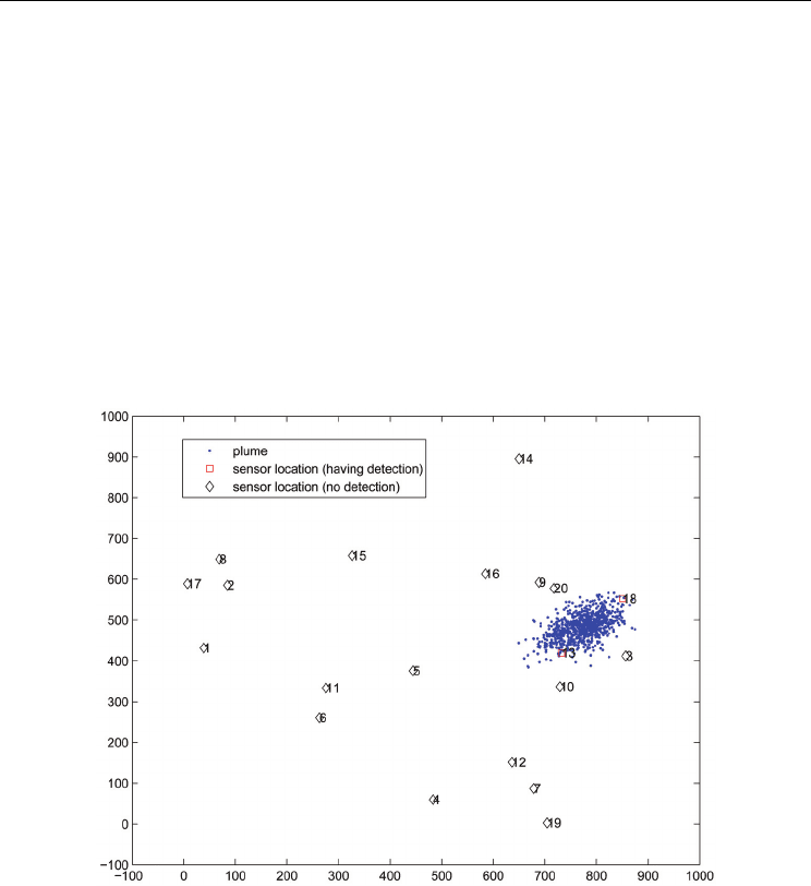
directly [18]. As an illustration, assuming Δt = 1s, the plume source is at (0, 0) with release

rate 100 particles per second and duration of 8s. There are 20 sensors randomly deployed in

a 1000×1000m

field with sensing range of 50m for each sensor and at least 10 particles in its

sensing area for a plume detection at any time. With wind velocity given by (v

(k), v

(k)) =

(8, 5)m/s, longitudinal and transversal dispersivity 

= 0.8, 

= 0.2 and diffusion coefficient

D = 0.9, one realization of the Gaussian plume at 100s is shown in Fig. 1 with two sensor

detections.

Fig. 1. One realization of plume propagation at K = 100.

We partition the region into 100 cells of the same square shape. It is assumed that initially

there is no plume source in the sensing field. All 20 sensors are assumed to be synchronized

and provide binary detections to a centralized data processor for plume mapping. The

FHMM assumes p

= 0.005 and p

= 0.8. The plume source always starts at the bottom left cell

at 4s with a constant release rate. Viterbi algorithm maintains all feasible solutions in its

trellis graph while greedy heuristic algorithm only keeps the solutions within a Hamming

distance of 8 to the initial candidate. We compare the probability of finding the correct cell

and initial releasing time of the plume source after K time steps. The plume localization

error probabilities are shown in Fig. 2 based on 5000 Monte Carlo runs for each K. We can

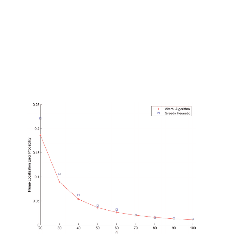
Advances in Greedy Algorithms

314

see that greedy heuristic algorithm has the localization error close to that using Viterbi

algorithm and the performance gap decreases as K increases. Using Matlab to compile both

algorithms on a Pentium 4 PC with 2.80GHz CPU, we found that the average time to find

the best state sequence using greedy heuristic algorithm is 0.05s when K = 100 while Viterbi

algorithm takes 5.3s in average to obtain the most likely sequence estimate. Thus the

proposed greedy algorithm achieves the plume localization accuracy close to that using

Viterbi algorithm while the computational time is orders faster than that using Viterbi

algorithm.

Our approach can also be used to estimate the total mass of plume release. However, there

is no guarantee on its accuracy even for instantaneous release of a single plume due to the

nature of binary sensor detection. To estimate the release rate sequence of a plume source,

denser sensor coverage or more accurate plume concentration intensity measurement is

needed. This problem will be addressed in the next section.

Fig. 2. Comparison of plume localization error probability with various observation length K.

3. Parameter estimation and model selection for gaussian plume sources

This section deals with joint plume localization and release sequence estimation when the

number of plume sources is unknown. We start with the plume source aggregation and

sensor measurement model in Section 3.1. Section 3.2 presents the regularized least squares

solution to the parameter estimation problem. Section 3.3 discusses the implementation of

the joint model selection (on the number of sources) and parameter estimation using greedy

algorithm and the choice of regularization parameter. Section 3.4 compares our approach

with alternative regularization methods. Section 3.5 provides realistic source release

scenarios to assess the performance of the proposed algorithm.

Greedy Methods in Plume Detection, Localization and Tracking

315

3.1 Plume aggregation and sensor measurement model

We assume that the wind field in the search area can be accurately modeled and sensors can

collect fairly accurate concentration readings in their neighboring areas. A Cartesian

coordinate system is used with x-axis oriented towards the mean wind direction, y-axis in

the cross-wind direction and z-axis in the vertical direction. If the source of a pollutant is

located at (x

, y

, z

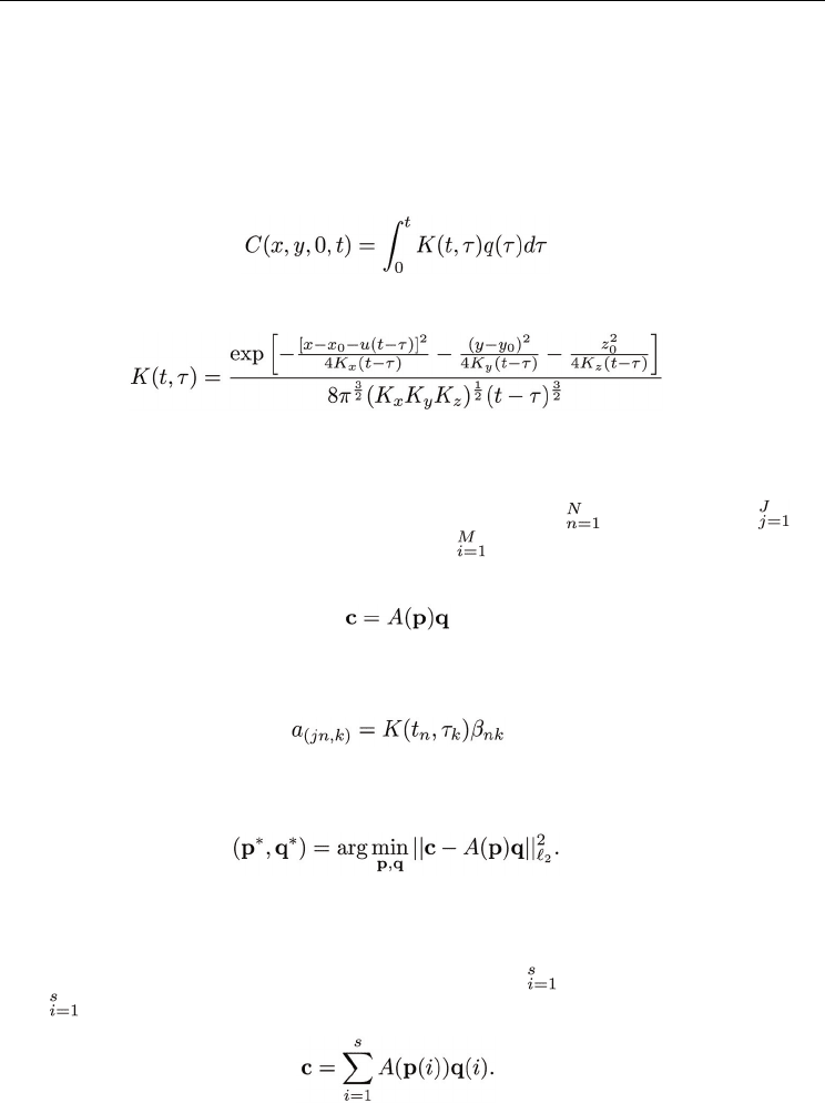
) with release rate q(t), then at time t, the concentration of the pollutant at

some down-stream location (x, y, 0) can be written as [16]

(19)

where the kernel K(t, τ ) is

(20)

with mean wind speed u and diffusion coefficients K

, K

along x, y and z directions,

respectively.

We assume that there are J sensors deployed at fixed locations where sensor j is located at

, y

, 0) and collects N concentration readings c

= {C(x

, y

, 0, t

)} . Denote by c = {c

} the

collection of all sensor readings. Denote by q = {q(τ

)} the discretized source release sequence

where q(τ

) is the release rate at time τ

. Ideally, we have the following observation equation

(21)

where p = (x

, y

, z

) denotes the unknown source location. Note that for measurement c

, 0, t

), the corresponding element a

(jn,k)

in A(p) is given by

(22)

where β

is a quadrature weight [16, 17]. The estimation of source location p and release rate

q can be formulated as the least squares problem given by

(23)

Note that this formulation is valid only for a single source.

To extend the estimation problem to include multiple sources, we assume that the

concentration readings are the results of aggregation from multiple source releases. Assume

that there are s sources with unknown locations {p(i)}

and release rate sequences

{q(i)} . Then we have the following ideal observation equation

(24)

The source parameter estimation problem becomes identifying the number of sources, the

corresponding origins and the release sequences jointly using only the concentration

readings from multiple sensors.

Advances in Greedy Algorithms

316

3.2 Regularized least squares

In the single source case, the matrix A in (23) can be analyzed for various source locations.

By ranking the singular values of A, the authors of [16] found that the discrete time least

squares problem (23) is in general ill-posed and suggested to use the Tikhonov

regularization to ensure certain smoothness of q. However, for a source with an

instantaneous release, the sequence q may have only a single spike, which violates the

smoothness assumption. Nevertheless, for multiple sources with instantaneous releases, we

will observe the aggregated sparse signal with an unknown number of spikes. In fact, the

sparsity assumption is crucial for the identification of multiple sources with instantaneous

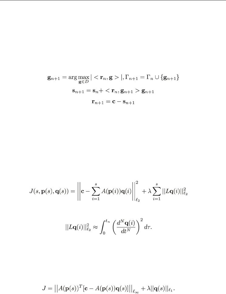
releases at different times. To encourage the sparsity of the release rate sequence estimate,

we propose to use l

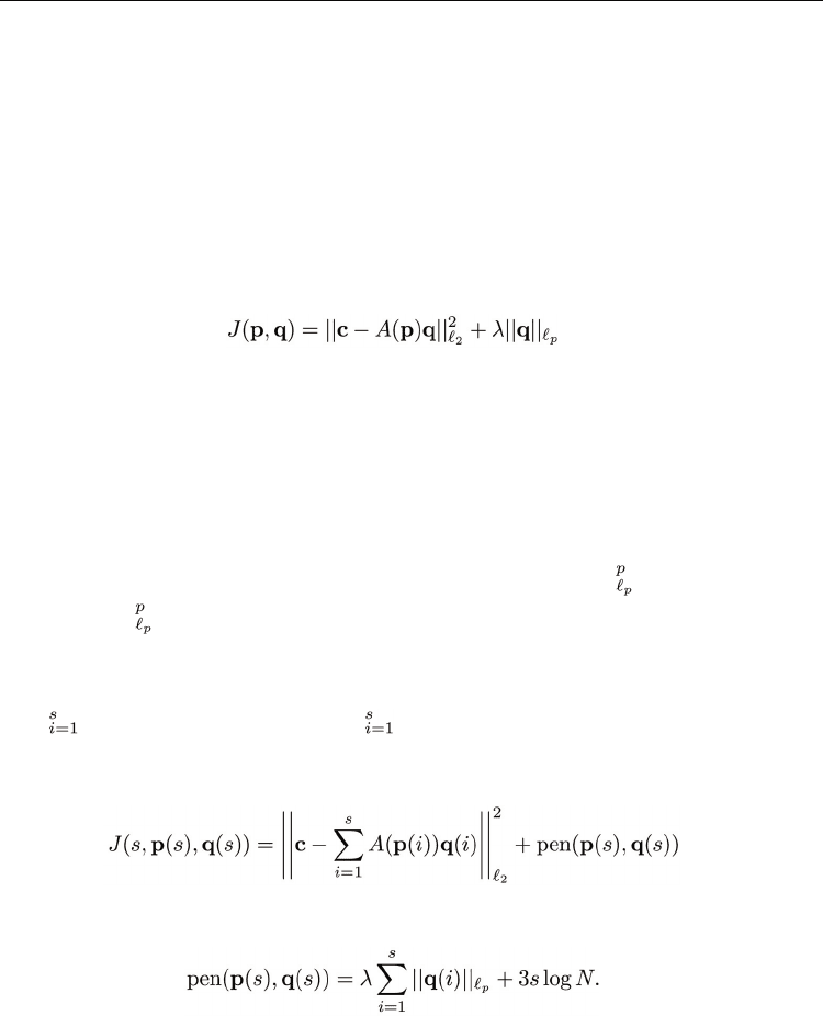
-regularized least squares as the objective function, i.e.,

(25)

where the regularization parameters p controls the sparsity of the solution q and λ makes

the tradeoff between the goodness-of-fit to the observations and the complexity of the

model. Note that p = 1 is popularly used in compressed sensing [10] due to its numerical

reliability. In fact, for any given p, minimizing (25) becomes a convex program if one

chooses p = 1. However, our l

-regularized least squares problem still requires non-convex

optimization without knowing the source location p. In addition, when choosing the

regularization term with 0 < p < 1, one favors a more sparse solution than that using l

regularization [7]. This might be helpful when one has prior knowledge about the type of

release of plume sources. In this case, the regularization term &· &

is not a norm, but

d(x, y) = &x - y&

is still a metric.

When the concentration readings are the aggregation of individual release, we have to

identify the number of sources and find their locations. In this case, we are facing a model

selection problem, where model s corresponds to s sources with unknown locations

{p(i)}

and release rate sequences {q(i)} . Assuming that different sources have different

instantaneous release times so that there is no identifiability issue among the models, we can

choose model s that minimizes a modified version of (25)

(26)

where

(27)

Note that the first term in the penalty encourages the sparsity of each identified source

release sequence and the second term is for model complexity of the source location

parameter based on the Bayesian information criterion [27]. The second term is necessary

because one does not want to treat one source with two instantaneous releases (sparsity of 2)

as two different sources with instantaneous releases at different time instances (sparsity of

1). In practice, when the locations of two sources are close, they could be identified as a

Greedy Methods in Plume Detection, Localization and Tracking

317

single source with aggregated release rate sequence. This seems to be acceptable when the

locations of multiple sources are within the arrange of the localization accuracy obtained by

minimizing (26).

3.3 Model selection and parameter estimation with a greedy algorithm

Finding the optimal solution to (26) requires solving a high dimensional nonlinear

optimization problem for any fixed regularization parameters p and λ. In practice, the

number of sources is usually small and a strong source can have the dominant effect on the

sensor readings. Thus it would be meaningful to identify and localize one source at a time

by treating the impact from the remaining possible sources as additive noise. In this case,

assuming the source location is given, one can obtain the sparse solution of the release rate

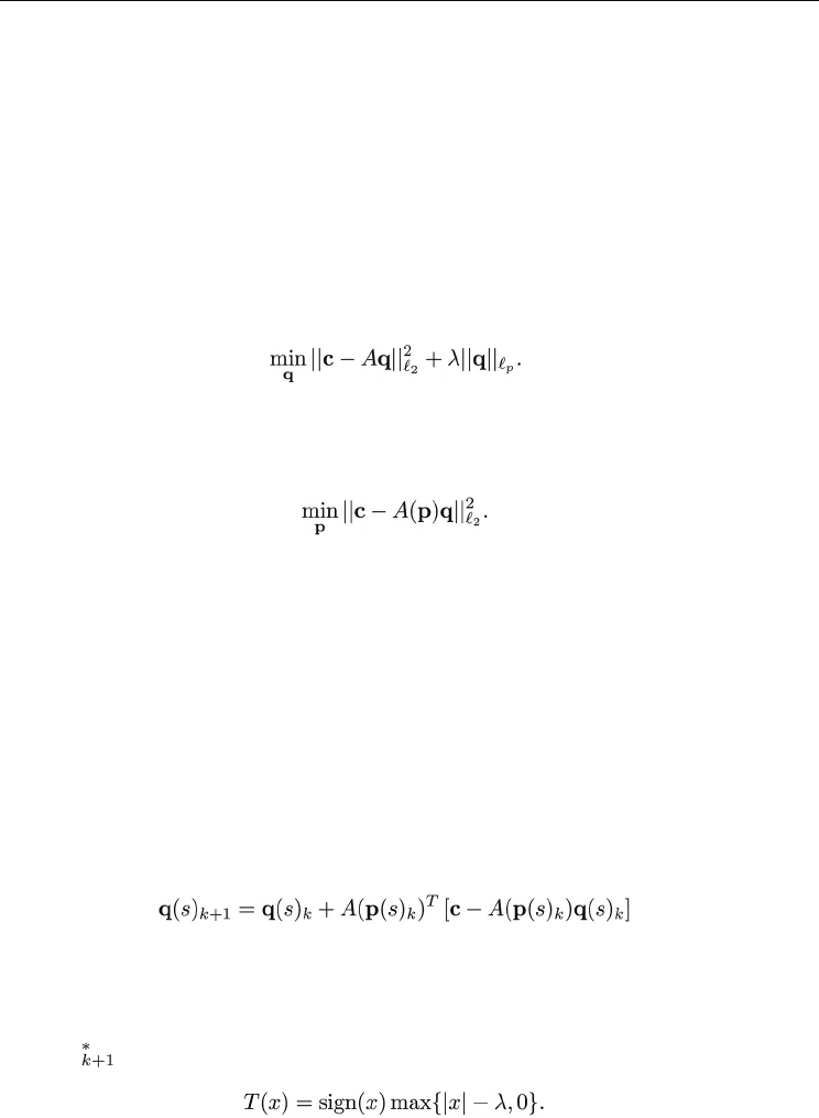
sequence by solving the following optimization problem.

(28)

When p = 1, the problem becomes a convex program and is highly related to LASSO [29].

Once we obtain the release rate of the source, we can refine the estimate of source location

by solving the regular nonlinear least squares problem given by

(29)

Note that for the newly estimated source location, the sparsity (non-zero locations) of the

solution to (28) may change. We can iteratively update the release rate and source location

estimate until the residual is comparable to the noise level of sensor readings.

We can extend the above procedure to deal with unknown number of sources. We apply a

greedy heuristic algorithm that iteratively refines the estimate of signal sparsity and the

noise level to determine the appropriate regularization parameter. The algorithm is greedy

in the sense of extracting one plume source at a time, from the strongest one to the weakest

(based on the penalty term in the model selection criterion). It simultaneously determines

the number of sources, the corresponding locations and release rate sequences by the

following steps.

1. Set s = 1.

2. Initialization: Set k = 0, q(s)

= 0 with an initial guess of source location p(s)

3. Refining the estimate: Use Newton-Ralphson update

(30)

to refine the estimated source release sequence.

4. Choosing regularization parameter: Compute the median of the residual

⏐c - A(p(s)

)q(s)

k+1

⏐ and choose λ proportional to the estimated noise level.

5. Denoising by soft thresholding: Compute the sparse approximation of q(s)

k+1

q(s)

=T(q(s)

k+1

) where

(31)

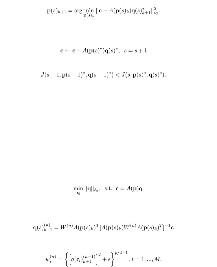
6. Source localization: Solve the nonlinear least squares problem

Advances in Greedy Algorithms

318

(32)

7. Model selection: Set k = k+1 and iterate until q(s) converges to a sparse solution q(s)* or

a predetermined maximum number of iterations k

max

has reached. Subtract out the

identified source from sensor readings.

(33)

Repeat steps 2-6 until

(34)

8. Declare the number of sources (s - 1), the corresponding locations p(s - 1)* and release

rate sequences q(s - 1)*.

For any given λ and p(s)*, the above iterative procedure converges to the optimal solution of

(28) for p = 1 [1]. We used the median estimator of the residue to obtain the noise level

which is robust against outliers. It is less sensitive to possible model mismatch than using

the mean of the residue when we initially assume that there is a single (strong) source which

results in the concentration readings while treating other (weak) sources as noise. Note that

the dimension of p(s) only depends on the model order, i.e., the number of sources, which is

usually much lower than the dimension of release sequences q(s). Thus solving the

nonlinear least squares problem (32) is less computationally demanding than solving (26)

directly.

When 0 < p < 1, (28) becomes non-convex program and any iterative procedure may be

trapped at a local minimum. Another issue is that (24) may become underdetermined when

A has rank deficiency. In such a case, the sparse solution to the following constrained

optimization problem

is still meaningful. To encourage more sparsity of the release rate sequence with smaller p

and solve the above constrained optimization problem directly, we apply iterative

reweighted least squares (IRLS) update [7] and replace the soft thresholding step by

(35)

where the weighting matrix W

(n)

is diagonal with entries

(36)

The damping coefficient ε is chosen to be relatively large initially and decreases to a very

small number when the above iteration is close to converge. Note that the IRLS algorithm

converges in less than 100 iterations most of the time in our simulation study. Even though

there is no theoretical guarantee that the resulting solution is globally optimal, we suspect

that it does approach to near global minimum since the solution quality improves when

using smaller p.

Greedy Methods in Plume Detection, Localization and Tracking

319

The above greedy algorithm can be interpreted as performing basis pursuit [13]. Specifically,

given the stacked observation c, we want to find a good n term approximation using

different sources as the basis functions from a general dictionary D. Denote by {g

} the i-th

basis being selected. Basis pursuit proceeds as follows.

1. Initialization:

• Approximation: s

= 0

• Residual: r

= c

• Basis collection: Γ

2. Pure greedy search:

Unfortunately, identifying a basis in the greedy pursuit is equivalent to localizing the origin

of a single source, which requires solving a nonlinear least squares problem. The

regularization on release rate sequence and penalty on the number of unknown sources

prevent the resulting optimization problem from being ill-posed. Note that when the basis

functions in the dictionary satisfy certain mutual incoherence property, the greedy basis

pursuit algorithm guarantees finding the best n term approximation [13].

3.4 Comparison with other regularization techniques

Tikhonov's regularization has been proposed in [16, 17] which essentially uses the objective

function

(37)

where L controls the smoothness of q(i) with the approximate form

(38)

The popular choice for obtaining a smooth solution is N = 2. Unfortunately, the above

regularization technique only works for continuous releases from well separated sources.

We rely on the sparsity of q(s) to identify the model order s, which is suitable for localizing

multiple sources of instantaneous release type.

Another sparsity enforced estimator was proposed in [4] which essentially minimizes the

following objective function

(39)

For known source locations, the estimated release rate guarantees to recover all possible

sparse signals with a large probability [4]. However, the above objective function is a non-

smooth function of p(s), which is difficult to optimize when both source locations and

release rate sequences are unknown. In practice, we fix the source locations p(s) and solve

Advances in Greedy Algorithms

320

(39) via linear programming. Then we fix the release rate sequence q(s) and update p(s) in

its gradient descent direction. The iteration continues until p(s) reaches a stationary solution

and the sparsity of q(s) does not change.

3.5 Simulation of joint plume localization and release sequence estimation

We present the simulation study of source localization and release rate estimation using

multiple sensors. We are interested in both model selection and source parameter estimation

accuracy.

3.5.1 Scenario generation

Consider a single source located at (-40, 35, 12) with instantaneous release of q(10) = 2 · 10

We assume that the wind speed u = 1.8 along x-axis and K

= K

= 12, K

= 0.2113. Five

sensors, located at (0, 0), (15, 15), (30, 30), (45, 45), (60, 60), respectively, collect concentration

readings synchronously with 100 samples per sensor. All sensors are on the ground with

zero elevation. We add Gaussian noise to the sensor readings with standard deviation

4 · 10

-3

. Each sensor will have a plume detection when the concentration reading exceeds

0.01. Fig. 3 shows one realization of the concentration readings from the five sensors. We can

see that sensor 1 has early detection while sensors 3-5 have relatively large peaks in the

concentration readings.

We also considered the case of two sources where one source located at (-40, 35, 12) has the

instantaneous release of q(10)=2 · 10

and the other located at (-30, 15, 15) has the

instantaneous release of q(50)=1 · 10

. Fig. 4 shows one realization of the concentration

readings from the five sensors. Compared with Fig. 3, we can barely see the effect of the

second source release due to the detection delay and source aggregation.

3.5.2 Model selection and parameter estimation accuracy

We want to compare our l

-regularization method with Tikhonov's method [16, 17] (denoted

by p = 2) and Dantzig selector [4] (denoted by p = ∞) for both one-source and two-source

cases. Note that Tikhonov's method is not appropriate for estimating instantaneous release

rate, which is non-smooth. However, it is meaningful to study how the incorrect assumption

in regularization may affect model selection accuracy. We estimated the probability of

identifying the correct number of sources based on 100 realizations of each case. For those

instances where the number of sources is correctly identified, we also computed the root

mean square (RMS) error of the location estimate for each source. In the case of s = 2, the

RMS error of the second source is in parentheses. The results are listed in Table 1. We can

see that in the single source case, our l

-regularization method can identify the correct

number of sources almost perfectly. In the two-source case, Tikhonov's method failed to

identify the second source most of the time and Dantzig selector can only identify the

correct number of sources with 64 out of 100 cases. Surprisingly, the proposed l

regularization method is able to find the correct model order with higher than 80%

probability. As we reduce p, there is a slight increase in the probability of obtaining the

correct number of sources due to the strong enforcement of sparsity. Among all cases where

the first source is correctly identified, the root mean square error of the estimated release

rate is 4.6 · 10

with p = 1. Note that the root mean square error of estimated location of the

first source increases when we have a second source aggregated to it. Note also that the

algorithm assuming the correct model order can only achieve the root mean square error of

estimated location of the second source around 18 using l

-regularized method with p = 1.