Balakumar Balachandran, Magrab E.B. Vibrations
Подождите немного. Документ загружается.

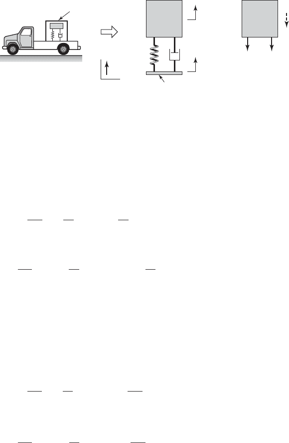
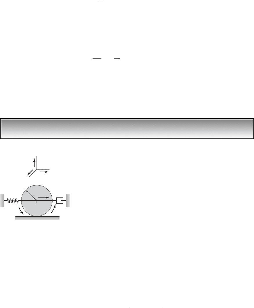
freedom system. The displacement response x(t) is measured from the sys-
tem’s static-equilibrium position. In the system shown in Figure 3.6, it is as-
sumed that no external force is applied directly to the mass; that is, f(t) 0.
Based on the free-body diagram shown in Figure 3.6, we use Eq. (3.1b) to
obtain the following governing equation of motion
(3.27)
which, on using Eqs. (3.14) and (3.18), takes the form
(3.28)
The displacements y(t) and x(t) are measured from a fixed point O located in
an inertial reference frame and a fixed point located at the system’s static-
equilibrium position, respectively. If the relative displacement is desired, then
we let
(3.29)
and Eq. (3.27) is written as
(3.30)
while Eq. (3.28) becomes
(3.31)
where y¨(t) is the acceleration of the base.
3.5.2 System with Unbalanced Rotating Mass
As discussed in Chapter 1, many rotating machines such as fans, clothes dryers,
internal combustion engines, and electric motors, have a certain degree of un-
balance. In modeling such systems as single degree-of-freedom systems, it is as-
sumed that the unbalance generates a force that acts on the system’s mass. This
d
2
z
dt
2
2zv
n
dz
dt
v
n
2
z
d
2
y
dt
2
m
d
2
z
dt
2
c
dz
dt
kz m
d
2
y
dt
2
z1t 2 x1t 2 y1t2
d
2
x
dt
2
2zv
n
dx
dt
v
2
n
x 2zv
n
dy
dt
v
2
n
y
m
d
2
x
dt
2
c
dx
dt
kx c
dy
dt
ky
90 CHAPTER 3 Single Degree-of-Freedom Systems
X
k c
O
Base
Package
x(t)
k(x y) c(x y)
..
mx
..
y(t)
j
Y
m m
FIGURE 3.6
Base excitation and the free-body diagram of the mass.
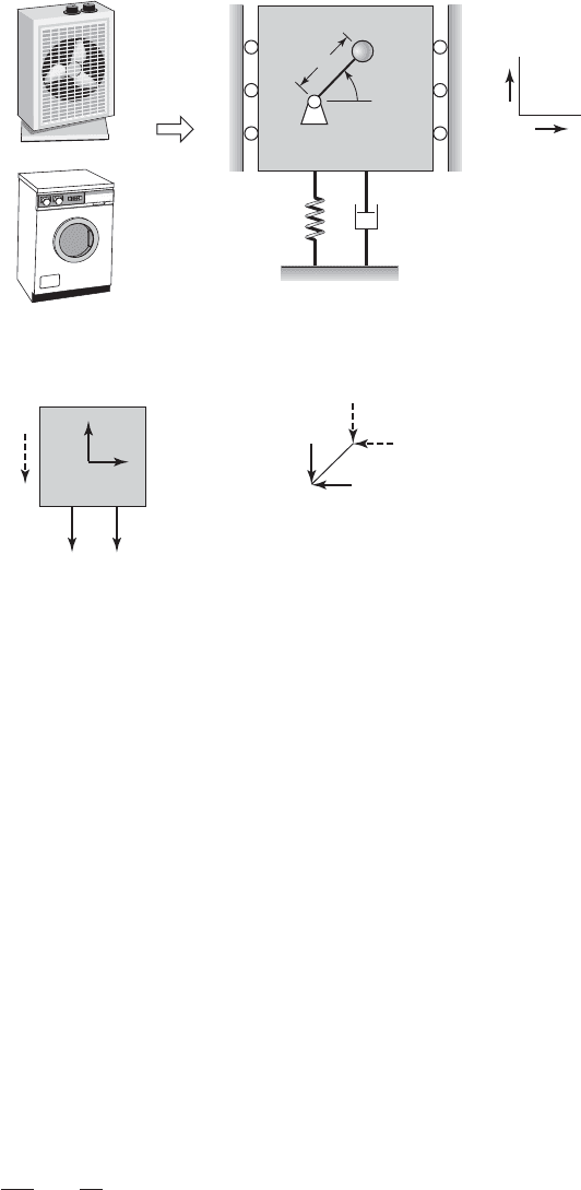
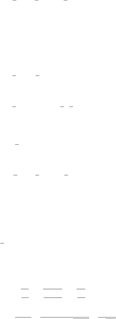
force, in turn, is transmitted through the spring and damper to the fixed base. The
unbalance is modeled as a mass m
o
that rotates with an angular speed v, and
this mass is located a fixed distance e from the center of rotation as shown in
Figure 3.7. Note that in Figure 3.7, M does not include the unbalance m
o
.
For deriving the governing equation, only motions along the vertical
direction are considered, since the presence of the lateral supports restrict
motion in the j direction. The displacement of the system x(t) is measured
from the system’s static-equilibrium position. The fixed point O is chosen to
coincide with the vertical position of the static-equilibrium position. Based
on the discussion in Section 3.2, gravity loading is not explicitly taken into
account.
From the free-body diagram of the unbalanced mass m
o
, we find that the
reactions at the point O are given by
(3.32)
and from the free-body diagram of mass M we find that
(3.33)M
d
2
x
dt
2
c
dx
dt
kx N
x
N
y
m
o
Pv
2
cos vt
N
x
m
o
1x
$
Pv
2
sin vt2
3.5 Governing Equations for Different Types of Applied Forces 91
kxcx
.
ck
Y
X
O'
O'
Fan
Clothes
dryer
O
O'
i
j
M
m
o
N
x
N
y
N
x
N
y
M
Mx
..
m
o
(x
2
sin t)
..
m
o
2
cos t
t
FIGURE 3.7
System with unbalanced rotating mass and free-body diagrams.
Then, substituting for N
x
from Eqs. (3.32) into Eq. (3.33), we arrive at the
equation of motion
(3.34)
which is rewritten as
(3.35)
where
(3.36)
In Eqs. (3.35) and (3.36), F(v) is the magnitude of the unbalanced force. This
magnitude depends on the unbalanced mass m
o
and it is proportional to the
square of the excitation frequency. From Eq. (3.6), it follows that the static
displacement of the spring is
(3.37)
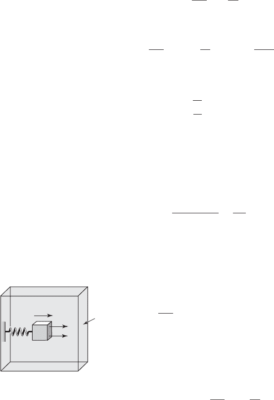
3.5.3 System with Added Mass Due to a Fluid
Consider a rigid body that is connected to a spring as shown in Figure 3.8. The
entire system is immersed in a fluid. From Eq. (3.8) and Figure 3.8, and noting
that c 0 because there is no damper, the equation of motion of the system is
(3.38)
where x(t) is measured from the unstretched position of the spring, f(t) is the
externally applied force, and f
1
(t) is the force exerted by the fluid on the mass
due to the motion of the mass. The force generated by the fluid on the rigid
body is
8
(3.39)
where M is the mass of the fluid displaced by the body, K
o
is an added mass
coefficient that is a function of the shape of the rigid body and the shape and
size of the container holding the fluid, and C
f
is a positive fluid damping co-
efficient that is a function of the shape of the rigid body, the kinematic vis-
cosity of the fluid, and the frequency of oscillation of the rigid body.
f
1
1t 2K
o
M
d
2
x
dt
2
C
f
dx
dt
m
d
2
x
dt
2
kx f 1t 2 f
1
1t 2
d
st
1M m
o
2g
k
mg
k
F1v 2 m
o
Pv
2
v
n
B
k
m
m M m
o
d
2
x
dt
2
2zv
n
dx
dt
v
n
2
x
F1v2
m
sin vt
1M m
o
2
d
2
x
dt
2
c
dx
dt
kx m
o
Pv
2
sin vt
92 CHAPTER 3 Single Degree-of-Freedom Systems
8
K. G. McConnell and D. F. Young, “Added mass of a sphere in a bounded viscous fluid,”
J. Engrg. Mech. Div., Proc. ASCE, Vol. 91, No. 4, pp. 147–164 (1965).
k
m
Fluid
Container
f
1
(t)
f(t)
x(t)
FIGURE 3.8
Vibrations of a system immersed in
a fluid.

After substituting Eq. (3.39) into Eq. (3.38), we obtain the governing
equation of motion
(3.40)
where K
o
M is the added mass due to the fluid. From Eq. (3.40), we see that
placing a single degree-of-freedom system in a fluid increases the total mass
of the system and adds viscous damping to the system.
9
A practical applica-
tion of the fluid mass loading is in modeling offshore structures.
10
In this section, the use of force-balance and moment-balance methods for
deriving the governing equation of a single degree-of-freedom system was il-
lustrated. In the next section, a different method to obtain the governing equa-
tion of a single degree-of-freedom system is presented. This method is based
on Lagrange’s equations, where one makes use of scalar quantities such as ki-
netic energy and potential energy for obtaining the equation of motion.
3.6 LAGRANGE’S EQUATIONS
11
Lagrange’s equations can be derived from differential principles such as the
principle of virtual work and integral principles such as those discussed in
Chapter 9. We will not derive Lagrange’s equations here, but use these equa-
tions to obtain governing equations of holonomic
12
systems. We first present
Lagrange’s equations for a system with multiple degrees of freedom and
then apply them to vibratory systems modeled with a single degree of free-
dom. In Chapter 7, we illustrate how the governing equations of systems with
multiple degrees of freedom are determined by using Lagrange’s equations.
Let us consider a system with N degrees of freedom that is described by
a set of N generalized coordinates q
i
, i 1, 2, . . ., N. These coordinates are
unconstrained, independent coordinates; that is, they are not related to each
other by geometrical or kinematical conditions. Then, in terms of the chosen
generalized coordinates, Lagrange’s equations have the form
(3.41)
where are the generalized velocities, T is the kinetic energy of the system,
V is the potential energy of the system, D is the Rayleigh dissipation function,
q
#
j
d
dt
a
0T
0q
#
j
b
0T
0q
j
0D
0q
#
j
0V
0q
j
Q
j
j 1,2, . . . , N
1m K
o
M2
d
2
x
dt
2
C
f
dx
dt
kx f 1t 2
3.6 Lagrange’s Equations 93
9
A similar result is obtained when one considers the acoustic radiation loading on the mass, when
the surface of the mass is used as an acoustically radiating surface. See L. E. Kinsler and A. R.
Frey, Fundamentals of Acoustics, 2nd ed., John Wiley and Sons, NY, pp.180–183 (1962).
10
A. Us´cilowska and J. A. Kol
´
odzeij, “Free vibration of immersed column carrying a tip mass,”
J. Sound Vibration, Vol. 216, No. 1, pp. 147–157 (1998).
11
For a derivation of the Lagrange equations see D. T. Greenwood, Principles of Dynamics, Pren-
tice Hall, Upper Saddle River, NJ, 1988, Section 6-6.
12
As discussed in Chapter 1, holonomic systems are systems subjected to holonomic constraints,
which are integrable constraints. Geometric constraints discussed in Chapter 1 are in this category.

and Q
j
is the generalized force that appears in the jth equation. Let us suppose
that the system is composed of l bodies. Then, the generalized forces Q
j
are
given by
(3.42)
where F
l
and M
l
are the vector representations of the externally applied forces
and moments on the lth body, respectively, r
l
is the position vector to the lo-
cation where the force F
l
is applied, and
v
l
is the lth body’s angular velocity
about the axis along which the considered moment is applied. The “” sym-
bol in Eq. (3.42) indicates the scalar dot product of two vectors.
Linear Vibratory Systems
For vibratory systems with linear inertial characteristics, linear stiffness char-
acteristics, and linear viscous damping characteristics, the quantities T, V, and
D take the following form:
13
(3.43)
In Eqs. (3.43), each of the summations is carried out over the number of de-
grees of freedom N and the inertia coefficients m
jn
, the stiffness coefficients
k
jn
, and the damping coefficients c
jn
are positive quantities.
Single Degree-of-Freedom Systems
In this chapter we shall limit the discussion to the case when N 1, which is
the case of a single degree-of-freedom system. Then Eqs. (3.41) reduce to
(3.44)
where the generalized force is obtained from Eq. (3.42), which reduces to
(3.45)Q
1
a
l
F
l
#
0r
l
0q
1
a
l
M
l
#
0v
l
0q
#
1
d
dt
a
0T
0q
#
1
b
0T
0q
1
0D
0q
#
1
0V
0q
1
Q
1
D
1
2
a
N
j 1
a
N
n 1
c
jn
q
#
j
q
#
n
V
1
2
a
N
j 1
a
N
n 1
k
jn
q
j
q
n
T
1
2
a
N
j 1
a
N
n 1
m
jn
q
#
j
q
#
n
Q
j
a
l
F
l
#
0r
l
0q
j
a
l
M
l
#
0v
l
0q
#
j
94 CHAPTER 3 Single Degree-of-Freedom Systems
13
The quadratic forms shown for T, V, and D in Eqs. (3.43) are strictly valid for systems with lin-
ear characteristics. In addition, the kinetic energy T is not always a function of only velocities as
shown here. Systems in which the kinetic energy has the quadratic form shown in Eqs. (3.43) are
called natural systems. For a general system with holonomic constraints, Eqs. (3.41) will be used
directly in this book to obtain the governing equations.
Linear Single Degree-of-Freedom Systems
For linear single degree-of-freedom systems, the expressions for the system
kinetic energy, the system potential energy, and the system dissipation func-
tion given by Eqs. (3.43) reduce to
(3.46a)
Comparing the forms of the kinetic energy T, the potential energy V, and the
dissipation function D with the standard forms given in Chapter 2, we
find that
(3.46b)
where m
e
is the equivalent mass, k
e
is the equivalent stiffness, and c
e
is the
equivalent viscous damping; they are given by
(3.46c)
On substituting Eqs. (3.46) into Eq. (3.44), the result is
(3.47)
Thus, to obtain the governing equation of motion of a linear vibrating
system with viscous damping, one first obtains expressions for the system ki-
netic energy, system potential energy, and system dissipation function. If
these quantities can be grouped so that an equivalent mass, equivalent stiff-
ness, and equivalent damping can be identified, then, after the determination
m
e
q
$
1
c
e
q
#
1
k
e
q
1
Q
1
d
dt
1m
e
q
#
1
2 0 c
e
q
#
1
k
e
q
1
Q
1
0
0q
#
1
a
1
2
c
e
q
#
2
1
b
0
0q
1
a
1
2
k
e
q
2
1
b Q
1
d
dt
a
0
0q
#
1
a
1
2
m
e
q
#
2
1
bb
0
0q
1
a
1
2
m
e
q
#
2
1
b
c
e
c
11
k
e
k
11
m
e
m
11
D
1
2
c
e
q
#
2
1
V
1
2
k
e
q
2
1
T
1
2
m
e
q
#
2
1
D
1
2
a
1
j 1
a
1
n 1
c
jn
q
#
j
q
#
n
1
2
c
11
q
#
2
1
V
1
2
a
1
j 1
a
1
n 1
k
jn
q
j
q
n
1
2
k
11
q
#
2
1
T
1
2
a
1
j 1
a
1
n 1
m
jn
q
#
j
q
#
n
1
2
m
11
q
#
2
1
3.6 Lagrange’s Equations 95

of the generalized force, the governing equation is given by the last of
Eqs. (3.47). We see further from the definitions Eqs. (3.14) and (3.18) that
(3.48)
It is noted that depending on the choice of the generalized coordinate, the
determined equivalent inertia, equivalent stiffness, and equivalent damping
properties of a system will be different. In the rest of this section, the use of
the Lagrange equations is illustrated with eleven examples. As illustrated in
these examples, we use the last of Eqs. (3.47) to obtain the governing equa-
tions of motion if the system kinetic energy, system potential energy, and dis-
sipation function are in the form of Eqs. (3.46b); otherwise, we use Eq. (3.44)
directly to obtain the governing equation of motion.
It is noted that only the system displacements and velocities are needed
from the kinematics to use Lagrange’s method whereas, to use the force-balance
and moment-balance methods, one also needs system accelerations and has to
deal with internal forces. In addition, with the increasing use of symbolic ma-
nipulation programs, it has become more common to have these programs de-
rive the governing equations directly from the Lagrange’s equations.
EXAMPLE 3.9
Equation of motion for a linear single degree-of-freedom system
For the linear system of Figure 3.1, the equation of motion is derived by us-
ing Lagrange’s equations. After choosing the generalized coordinate to be x,
we determine the system kinetic energy, the system potential energy, and the
dissipation function for the system. From these quantities and the determined
generalized force, the governing equation of motion of the system is estab-
lished for motions about the static equilibrium position.
First, we identify the following
(a)
where j is the unit vector along the vertical direction. Making use of Eqs.
(3.45) and (a), we determine the generalized force as
(b)
From Eqs. (2.3) and (2.10), we find that the system kinetic energy and poten-
tial energy are, respectively,
(c)V
1
2
kx
2
T
1
2
mx
#
2
Q
1
a
l
F
l
#
0r
l
0q
j
0 f 1t2j
#
0x j
0x
f 1t 2
q
1
x, F
l
f 1t 2j, r
l
x j, and M
l
0
z
c
e
2m
e
v
n
c
e
22k
e
m
e
v
n
B
k
e
m
e
96 CHAPTER 3 Single Degree-of-Freedom Systems
and, from Eqs. (3.46), the dissipation function is
(d)
Comparing Eqs. (c) and (d) to Eqs. (3.46), we recognize that
(e)
Hence, from Eqs. (e) and the last of Eqs. (3.47), the governing equation of
motion has the form
(f)
which is identical to Eq. (3.8).
In the following examples, we show how the Lagrange equations can be
used to derive the governing equations for a wide range of single degree-of-
freedom systems.
EXAMPLE 3.10
Equation of motion for a system that translates and rotates
In Figure 3.9, a system that translates and rotates is illustrated. After choos-
ing a generalized coordinate, we construct the system kinetic energy, the sys-
tem potential energy, and the dissipation function, and then noting that they
are in the form of Eqs. (3.46), we determine the equivalent inertia, equivalent
stiffness, and equivalent damping coefficient. Based on these equivalent sys-
tem properties and the last of Eqs. (3.47), we obtain the governing equation
of motion of this system. We also determine the expressions for the natural
frequency and the damping factor.
As shown in Figure 3.9, the disc has a mass m and a mass moment of in-
ertia J
G
about its center G. The disc rolls without slipping. The horizontal
location of the fixed point O is chosen to coincide with the unstretched length
of the spring, and the horizontal translations of the center of mass of the disc
are measured from this point O. When the center of the disc translates an
amount x along the horizontal direction i, then x ru, where u is the corre-
sponding rotation of the disc about an axis parallel to k. We can choose either
x or u as the generalized coordinate and express the one that is not chosen in
terms of the other. Here, we choose u as the generalized coordinate. Further-
more, we recognize that
(a)
Then making use of Eqs. (3.45) and (a), we determine the generalized force
to be
(b)Q
1
a
l
M
l
#
0
l
0q
#
1
M1t 2k
#
0u
#
0u
#
k M1t 2
q
1
u, F
l
0, M
l
M1t 2k, and
l
u
#
k
m
d
2
x
dt
2
c
dx
dt
kx f 1t2
m
e
m,
k
e
k,
and
c
e
c
D
1
2
cx
#
2
3.6 Lagrange’s Equations 97
X
i
j
k
Y
Z
O
G
r
k
M(t)
c
x
m, J
G
FIGURE 3.9
Disc rolling and translating.
To determine the potential energy, we note that we have a linear spring.
Therefore, we make use of Eq. (2.10) and arrive at
(c)
From Eq. (c), we recognize the equivalent stiffness of the system to be
(d)
To determine the kinetic energy of the system, we make use of Eq. (1.23);
that is, the kinetic energy of the disc is the sum of the kinetic energy due to
translation of the center of mass of the disc and the kinetic energy due to ro-
tation about the center of mass. Thus, we find that
(e)
where from Table 2.2, we have used J
G
mr
2
/2. From Eq. (e), we recognize
that the equivalent mass of the system is
(f)
In this case, the dissipation function takes the form
(g)
from which we identify the equivalent damping coefficient to be
(h)
Hence, from the determined generalized force and the equivalent inertia,
equivalent stiffness, equivalent damping properties, and the last of
Eqs. (3.47), we obtain the governing equation of motion
(i)
Natural Frequency and Damping Factor
To determine the natural frequency and the damping factor, we make use of
Eqs. (3.48) and find that
(j)z
c
e
2m
e
v
n
cr
2
213mr
2
/2 222k/3m
c
26km
v
n
B
k
e
m
e
B
kr
2
3mr
2
/2
B
2k
3m
3
2
mr
2
u
$
cr
2
u
#
kr
2
u M1t 2
c
e
cr
2
D
1
2
cx
#
2
1
2
c1ru
#
2
2
1
2
1cr
2
2u
#
2
m
e
3
2
mr
2
1
2
3mr
2
J
G
4u
#
2
1
2
c
3
2
mr
2
du
#
2
Rotational
kinetic energy
Translation
kinetic energy
T
1
2
mx
#
2
1
2
J
G
u
#
2
k
e
kr
2
V
1
2
kx
2
1
2
k1ru 2
2
1
2
kr
2
u
2
98 CHAPTER 3 Single Degree-of-Freedom Systems
⎫
⎬
⎭
⎫
⎬
⎭
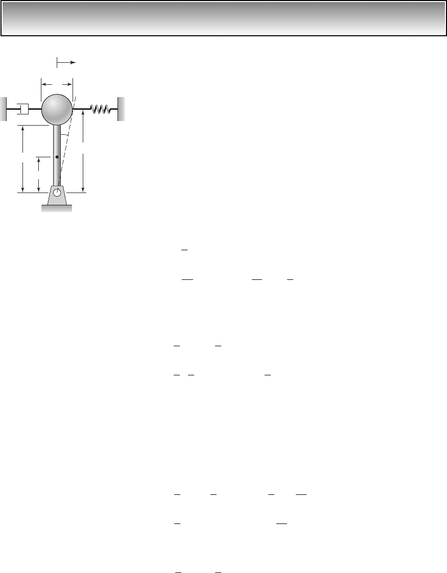
EXAMPLE 3.11 Governing equation for an inverted pendulum
For the inverted pendulum shown in Figure 3.10, we obtain the governing
equation of motion for “small” oscillations about the upright position. The nat-
ural frequency of the inverted pendulum is also determined and the natural fre-
quency of a related pendulum system is examined. In the system of Figure
3.10, the bar, which carries the sphere of mass m
1
, has a mass m
2
that is uni-
formly distributed along its length. A linear spring of stiffness k and a linear
viscous damper with a damping coefficient c are attached to the sphere.
Before constructing the system kinetic energy, we determine the mass
moments of inertia of the sphere of mass m
1
and the bar of mass m
2
about the
point O. The total rotary inertia of the system is given by
(a)
where J
O1
is the mass moment of inertia of m
1
about point O and J
O2
is the
mass moment of inertia of the bar about point O. Making use of Table 2.2
and the parallel-axes theorem, we find that
(b)
After choosing q
1
u as the generalized coordinate, and making use of
Eqs. (a) and (b), we find that the system kinetic energy takes the form
(c)
For “small” rotations about the upright position, we can express the
translation of mass m
1
as
(d)
Then, making use of Eqs. (2.10), (2.39), (2.45), and (d), the system potential
energy is constructed as
(e)
The dissipation function takes the form
(f)D
1
2
cx
#
1
2
1
2
cL
1
2
u
#
2
1
2
ckL
1
2
m
1
gL
1
m
2
g
L
2
2
du
2
V
1
2
kx
2
1
1
2
m
1
gL
1
u
2
1
2
m
2
g
L
2
2
u
2
x
1
L
1
u
1
2
c
2
5
m
1
r
2
m
1
L
1
2
1
3
m
2
L
2
2
du
#
2
T
1
2
J
O
u
#
2
1
2
3J
O1
J
O2
4u
#
2
J
O2
1
12
m
2
L
2
2
m
2
a
L
2
2
b
2
1
3
m
2
L
2
2
J
O1
2
5
m
1
r
2
m
1
L
1
2
J
O
J
O1
J
O2
3.6 Lagrange’s Equations 99
c
c.g.
k
m
2
O
x
1
L
1
L
2
r
2r
L
2
/2
L
2
m
1
FIGURE 3.10
Inverted planar pendulum restrained
by a spring and a viscous damper.