Amano R.S., Sunden B. (Eds.) Computational Fluid Dynamics and Heat Transfer: Emerging Topics

Подождите немного. Документ загружается.

Sunden CH002.tex 10/9/2010 15: 8 Page 46

46 Computational Fluid Dynamics and Heat Transfer

= u

x∗

+ Du



− p



) (61)

= v

y∗

+ Dv



− p



) (62)

= v

y∗

+ Dv



− p



) (63)

where u

, u

, v

, and v

are the corrected velocity components pertaining to CV.

Corresponding to the above corrected velocity components, the pressure at each

grid node is corrected to (p

∗



). Moreover, the asterisk superscript indicates

momentum-based velocity components and pressure. In equations (60)–(63), the

coefﬁcients Du

and Dv

are deﬁned as:



∂u

∂p



(64)



∂v

∂p



(65)

Similarexpressionsexistfor Du

andDv

. Substitutingequations(60)–(63) in

themasscontinuityequationofCV,thecorrespondingpressurecorrectionequation

can be obtained as follows:







− δ

(66)

where p



is the pressure correction of the main grid, while δ

is the excess mass

leaving control volume CV per unit time. It is deﬁned explicitly as:

= ρ

− ρ

+ ρ

− ρ

(67)

The ﬁnite-difference coefﬁcient a

stands for a

, a

, and a

, and can be

deﬁned as:

= ρ

(68)

= ρ

(69)

Similar expressions exist for a

and a

. The remaining pressure correction

equations for CV

,CV

, and CV

are similarly obtained as:







− δ

(70)







− δ

(71)







− δ

(72)

Sunden CH002.tex 10/9/2010 15: 8 Page 47

Higher-order numerical schemes for heat, mass, momentum transfer 47

Equations (52)–(57), (66), and (70)–(72) represent a complete set of ﬁnite-

differenceequationsforu,v,u



,andp



oftheNIMO

scheme.Theaboveﬁnite-differencepressurecorrectionequationsapplytoturbulent

ﬂowaswellastolaminarﬂow. However, themomentumﬁnite-differenceequations

for the turbulent ﬂow have extra source terms than their laminar counterparts.The

NIMO higher-order scheme will now be applied to steady laminar ﬂow in pipes

and 2D steady laminar ﬂow over a fence.

2.9.1 Steady laminar ﬂow in pipes

Equations(50)and(51)arethegoverningequationsforsteadylaminarﬂowinpipes

withconstant physicalproperties.Theexactanalyticalsolutionfor thistype ofﬂow

is a parabolic proﬁle for the fully developed axial velocity distribution along the

radial coordinate. It is given as:

= 2[1 −(r/R)

] (73)

where u

is the uniform axial velocity at the pipe entrance, r is the radial distance

from the pipe axis, and R is the pipe inner radius. Equation (73) is used here to

test the accuracy of the NIMO scheme. Equations (52)–(59), (67), and (70)–(72)

represent the NIMO ﬁnite-difference equations applicable to the laminar ﬂow in

pipes. The pipe radius R is taken as 1.0cm and the inlet uniform axial velocity is

1.0m/s. The ﬂowing gas is air at atmospheric pressure and 300K. For this ﬂow,

Reynoldsnumberis1,300.Thedimensionlesspipelength(L/D)is50.Thepressure

correction normal gradient, for each grid of the NIMO scheme, isequalto zero for

the fourboundaries of thesolution domain.Thisboundary conditionis validfor all

thetest problemsreported below. Zeronormalgradients ofall dependentvariables,

at the exit section, are imposed. Again this boundary condition is common to all

test problems reported below. The inlet axial velocity is 1.0m/s, while the radial

velocityisequalto zero.Atthepipewallthe velocity componentsareequaltozero.

However,atthepipeaxistheaxialvelocitygradientisequaltozero,whiletheradial

velocityitselfisequaltozero.Forauniform(80×80)grid,thenumberofiterations

is1,000,whichgivesanerrorlessthan0.1percentintheﬁnite-differenceequations.

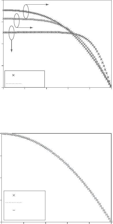
Figure 2.22 depicts the radial proﬁles of the dimensionless axial velocity for axial

distances (x/D)=2, 10, and 20.The axial velocityradialproﬁles for the main grid

andthex-gridareconsistent, showingcontinuousincreaseinthecenterlinevelocity.

Thefullydevelopedaxialvelocityradialproﬁles, showninFigure2.23forthegrids

of the NIMO scheme, are in excellent agreement with the exact analytical solution

given by equation(73). InFigures2.22 and2.23, u

isthe meanaxial velocity.The

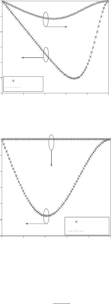
radialvelocityproﬁlesaredepictedinFigures2.24and2.25fordimensionlessaxial

distances of 2, 10, 20, and 50. It is interesting to noticethatthe maximum negative

radial velocity occurs at (x/D)=2; then it decreases sharply as the exit section

is approached. Figure 2. 26 shows the variations in the pressure along the axial

distance. The numerical results indicate that the pressure is uniformly declining

along the pipe length to overcome the laminar wall shear stresses.

Sunden CH002.tex 10/9/2010 15: 8 Page 48

48 Computational Fluid Dynamics and Heat Transfer

1.5

0.5

0.2 0.4 0.6 0.8

r /R

u/u

x/D = 2

x/D = 10

x/D = 20

Main grid

x-shifted

Figure 2.22. Dimensionless axial velocity proﬁles at different axial locations for

the laminar ﬂow in pipes with Re=1,300.

0 1

1.5

0.5

0.2 0.4 0.6 0.8

r/R

u/u

x/D  50

Main grid

x-shifted

Analytical

solution

Figure 2.23. Dimensionless axial velocity proﬁle for laminar ﬂow in a pipe with

Re=1,300.

2.9.2 Steady laminar ﬂow over a fence

This is a 2D steady laminar ﬂow over a single fence in a rectangular channel.

The ﬁnite-difference equations used in the laminar pipe ﬂow problem are also

applicabletoﬂow over afence. Excellentexperimentalresultswereobtained,using

laser-Doppler anemometry, by Carvalho et al. [13]. The ﬂow geometry used by

Sunden CH002.tex 10/9/2010 15: 8 Page 49

Higher-order numerical schemes for heat, mass, momentum transfer 49

−0.002

−0.012

−0.01

−0.008

−0.006

−0.004

0.2 0.4 0.6 0.8

r /R

v/u

x/D = 2

x/D = 10

Main grid

x-shifted

Figure 2.24. Dimensionless radial velocity proﬁles at different axial locations for

laminar ﬂow in pipes with Re=1,300.

−0.0012

0 0.2 0.4 0.6 0.8 1

−0.001

−0.0008

−0.0006

−0.0004

−0.0002

r /R

v/u

Main grid

x-shifted

x/D = 20

x/D = 50

Figure 2.25. Dimensionless radial velocity at different axial locations for laminar

ﬂow in pipes with Re=1,300.

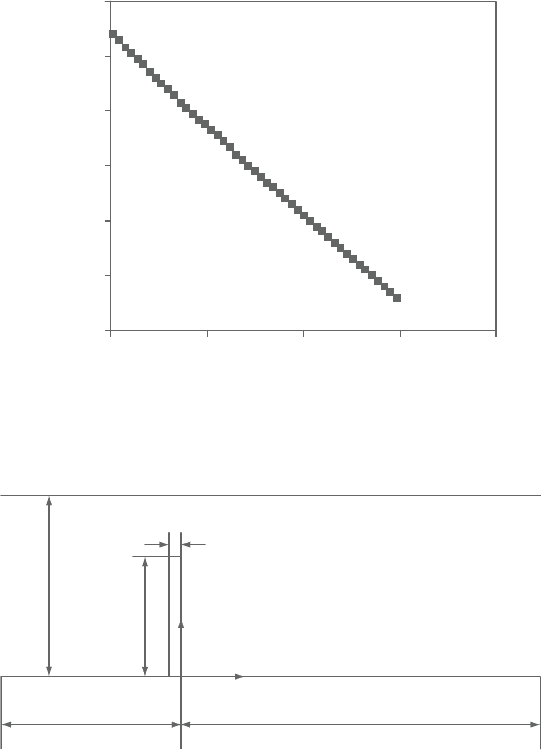
Carvalho et al. [13] is shown in Figure 2.27. The inlet velocity is prescribed as a

fully developed proﬁle for laminar ﬂow between two parallel plates, namely,

= 1.5



1 −



H − 2y





(74)

Sunden CH002.tex 10/9/2010 15: 8 Page 50

50 Computational Fluid Dynamics and Heat Transfer

−2.2

−2

−1.8

−1.6

−1.4

−1.2

−1

20 30 40 50 60

x/D

p − p

(N/m

)

Figure 2.26. Centerline axial pressure proﬁle in the laminar ﬂow in pipes with

Re=1,300.

5H 15H

0.1H

0.75H

Figure 2.27. Geometry of ﬂow over a fence.

whereu

andu

arethe velocityalong thex-axisat inletand itsmean value, respec-

tively.The distancefrom the lower plateis denoted by y, whilethe vertical distance

betweenthetwoplatesisgivenasH.Intheaboveequation,y rangesbetween0.0and

H.ThevalueofheightH isequalto1.0cm,andu

isequalto0.175m/s.Theﬂowing

gas isair at 300K.Theinlet Reynoldsnumber (Re) isequal to 82.5, which isbased

on u

and the fence height S(=0.75H). The thickness of the fence is 0.1cm. The

inletﬂowvelocityiscomputedfromequation(74), whilethetransversevelocity(v)

is equalto zero. Pressure correction nor mal gradients, u andv, are equal tozeroon

allsolidsurfacesoftheﬂowdomain. Forthislaminarﬂowproblems twogrids were

used,namely, (100×100)and(150×150).Toobtainnumericalerrorslessthan0.1

Sunden CH002.tex 10/9/2010 15: 8 Page 51

Higher-order numerical schemes for heat, mass, momentum transfer 51

0.25

0.5

0.75

(a)

x/S

y/H

Experimental data

100 × 100 grid

150 × 150 grid

−6.6 1.20−5.3

1.5

0.25

0.5

0.75

(b)

x/S

y/H

Experimetnal data

100 × 100 grid

150 × 150 grid

642

1.5

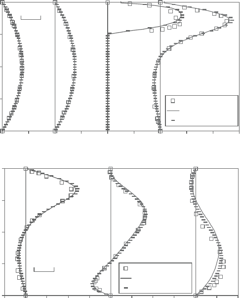
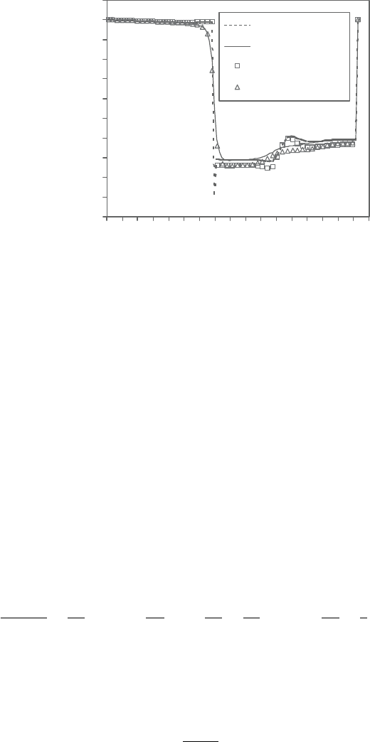
Figure 2.28. Comparisonbetweenpredictionsandmeasurementsofdimensionless

velocity along x-axis (u/u

) [13] for ﬂow over fence, Re=82.5.

percent,1,757and4,000iterationsareusedforthe(100×100)andthe(150×150)

grids,respectively.Thisshowsthatthenumberofiterationsforcompleteconversion

is more than doubled in the case of the ﬁner grid compared to the course one.

Thetransverseproﬁlesofthedimensionlessvelocitycomponentalongthex-axis

are depicted in Figure 2.28 for (x/S)=−6.6, −5.3, 0.0, 1.2, 2.0, 4.0, and 6.0. The

axial distance is measured from the fence. For (x/S)< 0.0 the (100×100) and the

(150×150)gridsgaveperfectﬁttotheexperimentaldata. However,for(x/S)< 0.0

the ﬁner grid gave excellent agreement with the experimental data. However, grids

ﬁner than (150×150) could not give any higher accuracy. Figure 2.28 shows that

the ﬂow direction is downward for 0.0< (x/S)< 4.0; then the gas ﬂows upwardly

for higher values of the distance along the x-axis. Recirculation zones are thus

created near the lower wall for (x/S)< 4.0 followed by recirculation zones at the

Sunden CH002.tex 10/9/2010 15: 8 Page 52

52 Computational Fluid Dynamics and Heat Transfer

x/s

−7

−1

−0.9

−0.8

−0.5

−0.4

−0.3

−0.2

−0.1

−0.6

−0.7

−3109876543210−1−2−4−6 −5

0.1

P − P

, N/m

y/H = 0,150 × 150

y/H = 1,100 × 100

y/H = 1,150 × 150

y/H = 0,100 × 100

Figure 2.29. Axial pressure proﬁles near the upper and lower walls for the ﬂow

over a fence with 100×100 and 150×150 girds, Re=82.5.

upper wall for higher values of (x/S). The radial pressure proﬁles along the x-axis

are plotted in Figure 2.29 for the (100×100) and (150×150) grids. The proﬁles

arechosen at(y/H)equal toapproximately0.0and1.0,respectively, nearthelower

and upper walls. It can be seen from this Figure that sudden pressure drop occurs

at the fence. However, it is smoother near the upper wall. Moreover, (100×100)

grid predicts lower pressure at the fence with respect to the (150×150) grid. It is

interestingtonoticethesuddenincreaseinpressureastheﬂowchangesitsdirection

in the vicinity of (x/H) ranging between 4 and 5.

2.10 Application of the NIMO Higher-Order Scheme to the

Turbulent Flow in Pipes

For constant-density steady turbulent ﬂow in pipes, the modeled time-mean

momentum equation can be written as follows:

∂(ρu

)

∂x

−

∂

∂x



(µ

+ µ)

∂u

∂x



=−

∂p

∂x

∂

∂x



(µ

+ µ)

∂u

∂x

−

ρkδ



(75)

where u

, u

, and p are time-mean values. The turbulent viscosity and turbulent

kinetic energy are denoted by µ

and k; in addition to time-mean momentum

equations, the time-mean mass continuity must be included.

∂(ρu

)

∂x

= 0 (76)

Sunden CH002.tex 10/9/2010 15: 8 Page 53

Higher-order numerical schemes for heat, mass, momentum transfer 53

The turbulent viscosity can be computed with the help of the two-equation

model ofturbulencefor the kinetic energy of turbulence(k) and itsdissipation rate

(ε). The governing equation for the kinetic energy of turbulence and its dissipa-

tion rate are written here such that they can be applied to the standard k-ε model

(Launder & Spalding [14]) and its low Reynolds number version of Launder and

Sharma [15].

∂

∂x

(ρu

k) −

∂

∂x



∂k

∂x



= G − ρ( ε + D) (77)

∂

∂x

(ρu

ε) −

∂

∂x



∂ε

∂x



= (C

G − C

ρε)

+ ρE (78)

where G



=µ

∂u

∂x



∂u

∂x

∂u

∂x



is the turbulent kinetic energy generation term and

is given by Launder and Spalding [14].The turbulent viscosity µ

is thus given as:

= C

ρk

/ε (79)

The high Reynolds number standard k-ε model is speciﬁed with the effec-

tive viscosity µ

=µ

, D =E =0.0, and f

=1.0. Moreover, the high

Reynolds number k-ε model logarithmic wall functions that prescribe at the wall

the shear stress, the generation term (G), and the value of ε are given by Launder

and Spalding [14].

However, the low Reynolds number k-ε model of Launder and Sharma [15]

takes the solution right to the pipe wall. The common constants between the two

versions of the k-ε model are given by Launder and Sharma [15] as c

=0.09,

=1.44, c

=1.92, σ

=1.0, and σ

=1.3. Moreover, the low Reynolds number

additional functions are deﬁned as follows [15]:

= exp[−3.4/(1 +R

/50)

] (80)

= 1.0 (81)

= 1 −0.3exp(−R

) (82)

D = 2(µ/ρ)



∂(k)

∂r



(83)

E = 2(µ/ρ)(µ

/ρ)



∂

∂r



(84)

where the turbulent Reynolds number R

is deﬁned as [15]:

= ρk

/(µε) (85)

Sunden CH002.tex 10/9/2010 15: 8 Page 54

54 Computational Fluid Dynamics and Heat Transfer

Equations (83) and (84) are given speciﬁcally for the turbulent ﬂow in pipes

where r is the radial distance and u is the axial velocity.

InthelowReynoldsnumbermodel, µ

isdeﬁnedas µ +µ

andthewallbound-

ary condition is deﬁned as ∂p



/∂r =u=v =k =ε =0.0. The boundary condition

at thecenterline is deﬁnedas∂φ/∂r =v =0, where φ stands forall dependent vari-

ablesexcept v.At the exit section, theaxial gradients ofall dependentvariablesare

equal to zero. At the inlet section, u =u

and v =∂p



/∂x =0, where u

is the inlet

uniform axial velocity.

The assessment of the accuracy of the results of the NIMO scheme is achieved

withthe helpofthe experimentaldataof Laufer[16]at Re=500,000and thesemi-

empirical relation obtained bySchlichting[17] for a large number of experimental

data forthefullydevelopedturbulent pipe ﬂow.The Schlichting 1/7thpower law is

given as [17]:

u/u



R −r



0 < r < 0.96R (86)

where u

is the fully developed centerline axial velocity.

The numerical predictions for turbulent ﬂow in pipes, using the NIMO higher-

order scheme, are shown in Figures 2.30–34. Air at 1.0 bar and 300K enters the

pipe at a uniform axial velocity of 29m/s. The pipe diameter is 24.7cm and its

dimensionless length (L/D) is equal to 30. For this ﬂow, the Reynolds number is

500,000. For the low and high Reynolds number turbulent models, a (100×100)

grid is used. The grid of the high Reynolds number model is uniform, while that

forthelowReynoldsnumbermodelconversestowardthepipewall.Forbothmodels

the number of iterations approximates 1,000, giving errors less than 0.1 percent in

the difference equations.

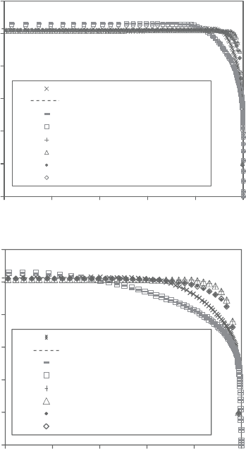
The developing turbulent ﬂow in pipes is depicted in Figure 2.30 for axial

distances(x/D)equalto2and5.Thedimensionlessaxialvelocity(u/u

)numerical

results of the main grid are essentially indistinguishable from those of the x-grid,

as can be seen from Figure 2.30. The near-wall region is shown in Figure 2.30b,

to facilitate the comparison of the wall effect as predicted by the low and high

Reynolds number models. The wall effect of the low Reynolds number model

propagates into the core of the turbulent ﬂow in pipes, while the high Reynolds

number model has its wall effect restricted to (r/R)> 0.95 for (x/D)< 5. More

developing ﬂow numerical results are shown in Figure 2.31 for (x/D) equal to

10 and 20. The high Reynolds number k-ε model wall effect is still conﬁned to

(r/R)> 0.75, while the low Reynolds number counterpart has its wall effect all

over the turbulent ﬂow for (x/D)=20. The dimensionless radial velocity (v/u

)

proﬁles are depicted in Figure 2.32, at (x/D)=5 and 20 and at the exit section.

The low Reynolds number model predicts higher absolute radial velocities, while

both models predictavanishing radial velocity at the fully developed ﬂow near the

exit section of (x/D)=30.The fully developed turbulent time-mean axial velocity

radial proﬁles are depicted in Figure 2.33, for the high and low Reynolds number

models. On the same ﬁgure, the measured fully-developed dimensionless axial

Sunden CH002.tex 10/9/2010 15: 8 Page 55

Higher-order numerical schemes for heat, mass, momentum transfer 55

0.2

0.4

0.6

0.8

1.2

0 0.2 0.4 0.6 0.8 1

Main grid, x /D = 2, lowRe

x-shifted, x /D = 2, low Re

Main grid, x /D = 5, lowRe

x-shifted, x /D = 5, low Re

Main grid, x /D = 2, high Re

x-shifted, x /D = 2, high Re

Main grid, x /D = 5, high Re

x-shifted, x /D = 5, high Re

r /R

u/u

0.2

0.4

0.6

0.8

1.2

0.75 0.8 0.85 0.9 0.95 1

r /R

u/u

Main grid, x /D = 2, low Re

x-shifted, x /D = 2, low Re

Main grid, x /D = 5, low Re

x-shifted, x /D = 5, low Re

Main grid, x /D = 2, high Re

x-shifted, x /D = 2, high Re

Main grid, x /D = 5, high Re

x-shifted, x /D = 5, high Re

(a)

(b)

Figure 2.30. Dimensionless axial velocity (u/u

) at different axial locations

for turbulent ﬂow in pipes with Re=500,000. (a) r/R from0to1.

(b) r/R from 0.75 to 1.

velocity [16] and the similar proﬁle that can be calculated by the semi-empirical

relation of Schlichting [17] are also plotted. The NIMO scheme predicts excellent

agreement with the fully developed axial velocity proﬁle given by the 1/7th power

lawofSchlichting[17]whenthelowReynoldsnumberk-ε modelisused.However,

the present numerical results for u/u

fall nicely between the experimental data

of Laufer [16] and the Schlichting’s 1/7th power law [17]. On the other hand, the

high Reynolds number model poorly predicts the fully developed turbulent pipe

ﬂow and hence should not be adopted for this type of ﬂow. Finally, the pressure

axial distributions, predicted using thelowand high Reynolds numberk-ε models,

are shown in Figure 2.34.This ﬁgure shows clearly that the absolute axial pressure