Ahsan A. Two Phase Flow, Phase Change and Numerical Modeling

Подождите немного. Документ загружается.

Heat Transfer and Phase Change in Deep CO

Injector for CO

Geological Storage

569

where α

thi

is the heat transfer coefficient at the inner wall of the tubing pipe, λ

is the heat

conductivity of the fluid (water) in the annulus, λ

Steal

is the heat conductivity of the casing

and tubing pipes, N

is the Nusselt number for the annulus and n is a correction number to

adjust the heat conductivity of the argon gas layer in the insulated tubing.

2.5 Evaluation of performance of thermal insulated tubing

Thermal insulated tubing pipe is sometime used for geo-thermal wells through cold

formation in order to prevent heat loss from produced hot spring water/steam. In case of

the Yubari injected CO

-ECBMR test, connected thermal insulated tubing pipes 20 m in

length were used partially in 2005-2006 and totally in 2007. The insulated tubing includes

argon gas shield layer is enclosed between inner and outer pipes to prevent heat loss from

inside ideally with low thermal conductivity of argon gas; 0.116 W/m°C. However, joints

between pipes are not shielded, and natural gas convection flow in the shield is expected to

make increase the heat loss trasfered from the flow to outer tubing.

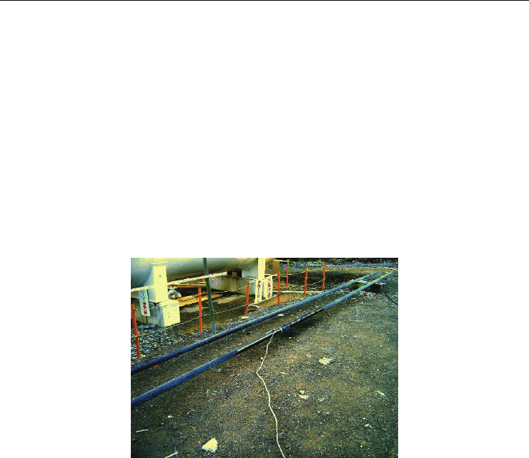
Fig. 4. Test to evaluate of equivalent thermal conductivity in the thermal insulated tubing

using by pulsed heating carried at Yubari CO

-ECBMR test field (Oct. 10, 2006) (see

Yasunami et al., 2010)

To evaluate the thermal performance of the insulated tubing, tests using a insulated tubing

pipe were carried out by pulsed heating from inside and measurements of outer and inner

surface temperatures of the pipe placed horizontally as shown Fig. 4. Furthermore, the

equivalent thermal conductivity was analyzed with Choukairy et al.’s equation (see section

2.5) and the history matching study for the well logging data. The thermal conductivity

correction factor for conductivity of argon gas, n, is evaluated as shown in Fig. 5.

The equivalent heat conductivity including inside convective heat transfer was evaluated as

three times larger as that of original argon gas without longitudinal heat loss through to

connected tubing pipes. The correction factor, n, was introduced to adjust the equivalent

heat conductivity of the tubing based on the original heat conductivity of argon gas. It was

determined to be n = 3 but heat loss through the joints that are between the insulated tubing

was not included in the test. The thermal equivalent conductivity of the insulated tubing

was determined to be n = 4 or λ = 0.21W/m°C based on the well logging temperature at the

Yubari CO

-ECBMR test site and the measurement data were obtained from the heater

response test carried out in the test field.

Two Phase Flow, Phase Change and Numerical Modeling

570

Fig. 5. Thermal conductivity correction factor for shielding with argon gas (*; spec value

provided by a steel pipe maker)

2.6 Convective heat transfer in the annulus

Natural convection of annulus fluids makes influences on the heat transfer rate from the

tubing pipe to the surrounding casing pipe and the formation. Choukairy et al. (2004)

presented the following formula for the Nusselt number, N

, for natural convection flow in

an annulus with various radius ratios:

1/4 5/4

()

uram

NPRT

== ⋅ (6)

where

denotes the natural convection heat transfer coefficient on the inner surface of the

casing, L (=r

cai

- r

tuo

) is the width of the annulus, κ is the radius ratio, m is a constant defined

by Choukairy et al., A is the aspect ratio, P

is the Prandtl number, R

is the Rayleigh number

and T

is a dimensionless temperature defined by following equations:

(7)

cai

tuo

= (8)

()

gT T h

αυ

−⋅

⋅

(9)

4/5

−

(10)

where h

is the circulation height of natural convection flow, g is the acceleration of gravity,

is the coefficient of thermal expansion of the fluid, υ

is the dynamic viscosity and

heat diffusivity of fluid in the annulus. The Nusselt number, N

, calculated by Eq.(4) was

used for each elevation.

Heat Transfer and Phase Change in Deep CO

Injector for CO

Geological Storage

571

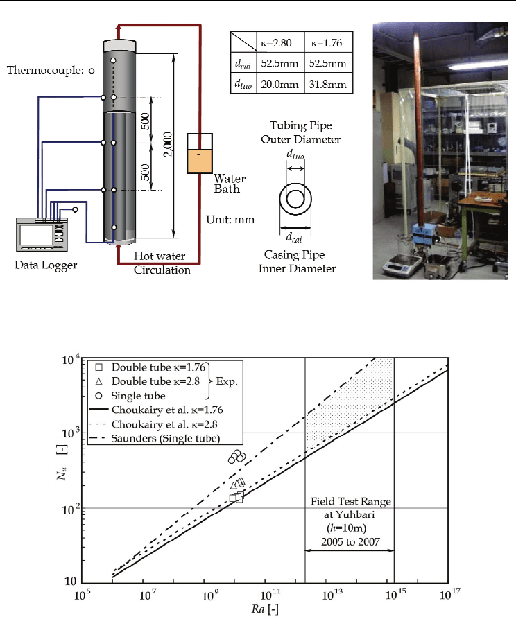
Fig. 6. Experimental setup to verify natural convection heat transfer coefficient in the

annulus (Yasunami et al., 2010)

Fig. 7. Experimental results of Nusselt number for convective heat transfer in annulus

(Yasunami et al., 2010)

Laboratory experiments were carried out to verify the reliability of Choukairy’s equation

and to investigate the heat transfer rate using the well models consisting of two copper

pipes with different diameters as shown in Fig. 6. Hot water at 40 to 60 °C was circulated

through the inner pipe instead of CO

. Pipe temperatures were measured by T-

thermocouples that were placed on the pipe surfaces. Figure 7 shows experimental results

Two Phase Flow, Phase Change and Numerical Modeling

572

obtained for N

and compared with those from Choukairy’s equation. In addition, measured

values of N

on the outer surface of the single tubing determined using the equation

proposed by Saunders [after Rohsenow et al. (1998)] were also compared in Fig. 7. Based on

these results, we have found that Choukairy’s equation is able to evaluate the heat transfer

rate in the annulus.

2.7 Unsteady casing temperature

On the other hand, the temperature of the formation outside the casing pipe (outer surface)

increases gradually after the injection. Assume T

is the initial strata formation temperature

and T

is the temperature in the annulus, the temperature at outer surface of the casing T

can be given by the solution for the unsteady heat conduction equation; Eq. (3). It has been

presented by Starfield and Bleloch (1983):

()

wan an

TT TT

=+ −

(11)

where η

is defined as the elapsed time factor and B

is the non-dimensional Biot number,

and B

is defined by following equation:

ca cao

⋅

= (12)

where

is the apparent heat transfer rate at the inner casing and λ

is the heat

conductivity of rock. Starfield and Bleloch (1983) reported equations for the elapsed time

factor η

, which is a function of the Fourier number, τ, and Sasaki & Dindiwe (2002)

revised

it for τ≤1.5 as:

1.5

[0.9879 0.3281(ln ) 0.03064(ln )

τη

ττ

≤=

(13)

1.5 10

[0.979813 0.383760(ln )

τη

≤≤ =

(14)

10 100

[0.839337 0.444718(ln )

τη

≤≤ =

(15)

2(1 )

1000

0.57722

τη

Λ−Λ−Λ−Λ

≤=

(16)

0.57722

[ln(4 ) 1.15444)

Λ=

−

(17)

cao

= (18)

The elapsed time factor η

vs. Fourier number

calculated by equations (13) to (18), is

presented in Fig. 8.

Heat Transfer and Phase Change in Deep CO

Injector for CO

Geological Storage

573

Fig. 8. Elapsed time factor vs. Fourier number

Fig. 9. CO

pressure-specific enthalpy and phase diagram calculated with PROPATH(2008)

for 10 to 100 °C and 1 to 100 MPa (○; Critical point; 31.1°C and 7.38MPa)

2.8 Numerical equations for the determination of the CO

specific enthalpy

Changes in CO

temperature and phase (gas, liquid and supercritical) are accompanied by a

specific enthalpy change. CO

specific enthalpy, E(P,T) may be expressed by:

(,) (1 )

E P T C dT V T dP

=+−



(19)

where V is the specific volume, β is the coefficient of thermal expansion, T

and P

are triple

point temperature (=-56.57°C) and pressure (=0.5185MPa). The diagram CO

pressure-

specific enthalpy for temperature range 10 to 100 °C and pressure range 1 to 100 MPa, that is

calculated by PROPATH(2008), is shown in Fig. 9.

The specific enthalpy of CO

decreases with depth x by heat loss from CO

flow to the

formation around the injection well.

2( )

TTx

πλ

Δ= − Δ

(20)

Two Phase Flow, Phase Change and Numerical Modeling

574

where T

is the CO

temperature in the tubing, ∆x is the length of the element and T

is the

temperature at the outer surface of the casing.

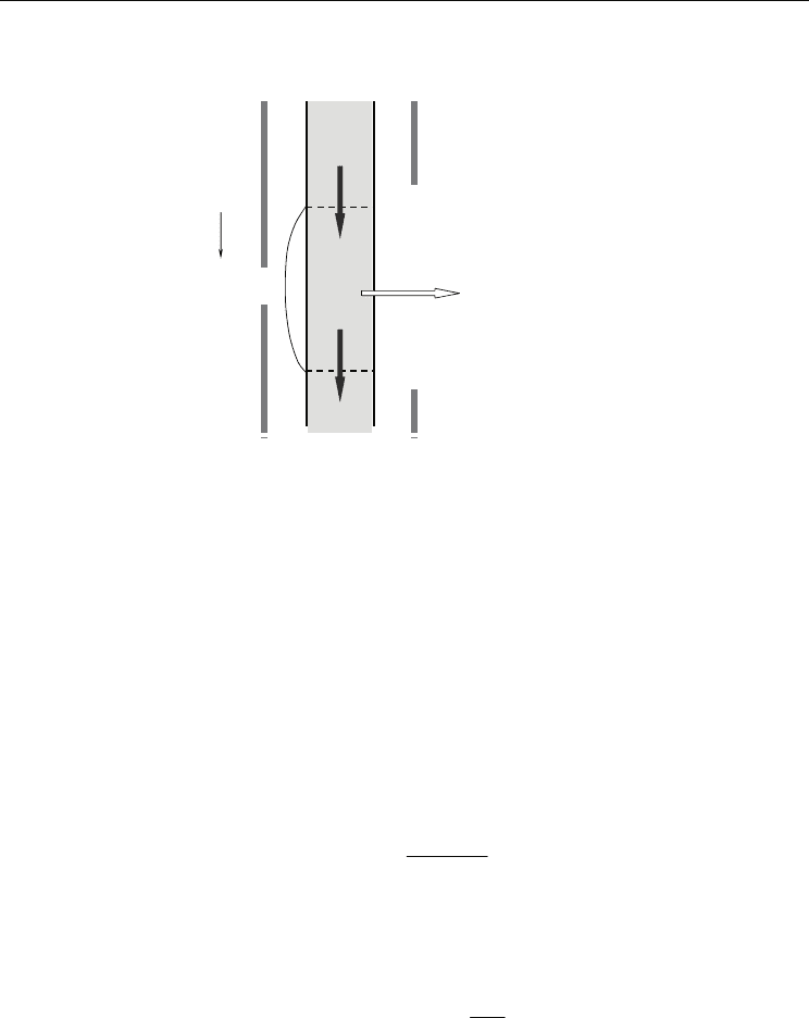
Heat Loss

Δq

i+1

, ρ

i+1

, E

i+1

, P

i+1

, ρ

, E

, P

i+1

+Δx/2)

Fig. 10. The numerical calculation model for CO

temperature and pressure in the injector

temperature T

was calculated using the function shown in Fig. 10. The function used to

calculate the temperature T

from the specific enthalpy E

and pressure P

is defined as:

(,)

iii

TEP

= (21)

The heat flow rate, Δq

, of a small element in the well, Δx

, may be written as:

2( )

iiiii

TTx

πλ

Δ= − Δ (22)

where λ

is the equivalent heat conductivity at x

, T

is the temperature of CO

in the tubing

and T

is the temperature of the casing outer surface at each element denoted i . The heat

generation by flow friction with internal surface of the tubing can be omitted due to very

small pipe friction factor and low fluid viscosity for CO

flow.

The specific enthalpy of CO

, E

i+1

at x

i+1

+Δx

is obtained from:

Δ−Δ

(23)

where M is the mass flow rate of CO

and ΔW is heat generated by a heater during x

to x

i+1

Using the function ρ(P

), calculation of the CO

density from P

and T

and the CO

pressure at x

i+1

, P

i+1

is given by;

(,)

ii ii i

tui

PP PT



=+ − Δ





(24)

where f and v are friction factor and average velocity of tubing pipe. Then the temperature

of CO

at x

i+1

can be obtained from:

111

(,)

iii

TEP

+++

= (25)

Heat Transfer and Phase Change in Deep CO

Injector for CO

Geological Storage

575

In these numerical simulations, E(P,T), θ(P,T) and ρ(P,T) and other fluids properties are

calculated using a corresponding software subroutines, such as PROPATH(Propath Group,

2008) and NIST (2007). Calculation step Δx

= 1.0m can be used to get enough accuracy

(Yasunami et al., 2010).

2.9 Required values in the numerical calculations

For these numerical calculations, three values for each depth are required.

1. Heat diffusivity of formation.

In Yubari ECBMR test project introduced in this book, no rock core drilling was carried

out from o m to -800 m, thus we had to estimate rock properties (Fujioka et al., 2010).

The heat conductivity λ

and the heat diffusivity a

of the rock formation outer casing

have not been measured previously, so values of a

=1.30×10

-6

/s and λ

=1.30 W/mK

were assumed and this was based on standard heat properties of sedimentary rocks

(Yasunami et al., 2010).

2. Circulation height of natural convection flow in the annulus.

It was difficult to measure the circulation height h of natural convection in the annulus

at the Yubari site. However, the bottom hole temperature was not sensitive to h, even

when h changed from 5 to 20 m. Thus h =10m was assumed as an appropriate value

since natural convection was not observed at lower than 2m in the experiments

described in the previous section.

3. Heat capacity of the tubing or casing.

We assumed that temperature changes of tubing and casing pipes were quasi-steady

and thus the heat capacity of these pipes was not included in the equations.

3. Results of Yubari ECBMR test project

3.1 Injection well formation

Figure 11 shows a well structure and formation used at the Yubari CO

-ECBMR test project

in 2005. CO

heat loss occurs during flow down to the bottom and propagates through

various cylindrical combinations of steels and fluids with various thermal properties in the

well configuration. Table 1 shows conditions used for the models from 2005 to 2007 carried

out in the project denoted as;

Model 2005:

The well was drilled in 2005 (hereafter denoted as Model 2005) and consisted of

thermally insulated tubing 180 m in length from the well head.

Model 2006:

In 2006, thermally insulated tubing of 180m in length was used at the head (0 to 180m)

and the bottom (650 to 890m) while the annulus was filled with liquid CO

Model 2007:

In 2007 all the injection pipe tubing was replaced with thermally insulated tubing of

890 m in length and H

O was used to fill the annulus. This was done to minimize heat

loss from the tubing and thus keep CO

in its supercritical condition.

Heater Model 2007:

To overcome the difficulty of low temperature and low injection rate, numerical predictions

were done considering the use of an electric line heater to heat up CO

flow at the

position of 180m from the surface. The heater capacity of W = 1.43kW was chosen because

of the cable strength and restrictions of materials against corrosion of supercritical CO

Two Phase Flow, Phase Change and Numerical Modeling

576

injection from evaporation plant

Well head

WH,

)

Water

Gas in Annulus

or CO

)

Single Tubing

Initial Strata

Temperature; T

(x)

Cement Sealing

Thermal Insulated

Tubing

Packer

(

= 890m

)

Bottom Hole

, P

)

Heater, W (kw)

(0)

(H)

Coal Seam

Fig. 11. An example of CO

injection well formation, initial strata temperature and schematic

annulus formation (Yubari CO

-ECBMR test project, Model 2005)

Term/Model

Model

2005

Model

2006

Model

2007

Model

2007+ Heater

Temp. and Press. At

well head (T

, P

)

70 ºC

9.0 MPa

70 ºC

9.0 MPa

70 ºC

8.6 MPa

70 ºC

8.6 MPa

S. Enthalpy at well head;

(kJ/kg)

766.34 766.34 771.27 771.27

Injection rate M(kg/day) 3000 3000 3000 11000

;

x=0~180m

Insulated

tube

Insulated

tube

Insulated

tube

Insulated

Tube

;

x=180~667m

Single

tube

Single

tube

Insulated

tube

Insulated

Tube

Tubing

;

x=690~890m

Single

tube

Insulated

tube

Insulated

tube

Insulated

Tube

for H

Gas Liquid CO

Water Water

for H

Gas Liquid CO

Water Water

Fluid in

annulus

for H

Water Water Water Water

Heater output; W(kW)

(x=0~255m)

0 0 0 1,430

Table 1. Parameters of injection well formation for CO

injection

Heat Transfer and Phase Change in Deep CO

Injector for CO

Geological Storage

577

3.2 Effect of natural convection in the annulus

The results of temperature prediction against depth after one day by the heat conduction

model (N

=1 and n=1) and the heat convection model for an injection temperature of 70°C,

an injection pressure of 9MPa and an injection rate of 3.0ton/day is shown in Fig. 12.

0 100 200 300 400 500 600 700 800 900

Depth x [m]

Temperature [ºC]

Initial strata temp.

Heat convection

Model

[n ＝4, Nu

(

)

]

Heat conduction model

(

n =1,

)

ection rate : M= 3000k

/da

Annulus : Liquid CO

ectionTemp. and Press. : 70 ºC and 9 MPa

Fig. 12. A comparison of CO

temperatures after 1 day between heat conduction and heat

convection models (Model 2005, 180m insulated tubing was partly used from well head)

Figure 13 shows comparisons of CO

temperature and pressure at the bottom hole.

Numerical simulation results for the data, obtained in 2005 at the Yubari field, show that the

heat convection model is better than the conduction model. This is because the temperature

of the CO

decreased by heat loss caused by natural convection in the annulus. The bottom

pressure increased because of the increase in CO

density that resulted from the CO

supercritical to liquid phase change.

Fig. 13. Comparisons of bottom hole temperature and pressure (BHT and BHP) that were

simulated by heat conduction and heat convection models with monitored values (Model

2005)

Two Phase Flow, Phase Change and Numerical Modeling

578

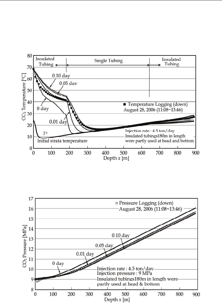
Figures 14 and 15 show comparisons of CO

temperature and pressure between simulations

and the well logging data for injection conditions of 68.54°C, 9MPa and 4.5ton/day at the

well head. Since logging from the surface to a level of -890m took 2.4hours (Prensky,1992),

simulated CO

temperatures against depth were plotted for each time segment. The reason

for the rise in the measured pressure near the well head of about of 0.3 MPa is unknown at

present.

Fig. 14. Comparison between logged temperature and simulation results for Model 2006

(Logging data was obtained on August 28, 2006 (11:08 to 13:46) at the Yubari ECBMR test

site)

Fig. 15. Comparison between logged pressure and simulation results (Model 2006)

(Logging data was obtained on August 28,2006 (11:08 to 13:46) at the Yubari test site)