Ablowitz M.A. Nonlinear Dispersive Waves: Asymptotic Analysis and Solitons
Подождите немного. Документ загружается.

2.6 Characteristics for first-order equations 25
we observe that u(x, t) = f (x + a
1
t). This solution can be checked directly by
substitution into the PDE.
We can also solve (2.4) using the so-called method of characteristics. We
can think of the left-hand side of (2.4) as a total derivative that is expanded
according to the chain rule. That is,
du
dt
=
∂u
∂t
+
dx
dt
∂u
∂x
= 0. (2.6)
It follows from (2.6) that du/dt = 0 along the curves dx/dt = −a
1
,or,said
differently, that u = c
2
, a constant, along the curves x + a
1
t = c
1
. Thus for the
initial value problem u(x, t = 0) = f (x), at any point x = ξ we can identify
the constant c
2
with f (ξ) and c
1
with ξ. Hence the solution to the initial value
problem is given by
u = f (x + a
1
t).
Alternatively, from (2.4) and (2.6) (solving for du), we can write the above
in the succinct form
dt
1
=
dx
−a
1
=
du
0
.
These equations imply that
t =
−1
a
1
x +
c
1
a
1
, u = c
2
,
where c
1
and c
2
are constants. Hence
x + a
1
t = c
1
, u = c
2
.
For first-order PDEs the solution has one arbitrary function degree of freedom
and the constants are related by this function. In this case c
2
= g(c
1
), where g
is an arbitrary function, leads to
u = g(x + a
1
t).
As above, suppose we specify the initial condition u(x, 0) = f (x). Then if we
take c
1
= ξ, so that t = 0 corresponds to the point x = ξ on the initial data, this
then implies that u(ξ, t) = g(ξ) = f (ξ); now in general, along ξ = x + a
1
t, that
agrees with the solution obtained by Fourier transforms. The meaning of ξ is
that of a characteristic curve (a line in this case) in the (x, t)-plane, along which
the solution is non-unique; in other words, along a characteristic ξ, the solution
can be specified arbitrarily. Moreover as we move from one characteristic, say
ξ
1
, to another, say ξ
2
, the solution can change abruptly.

26 Linear and nonlinear wave equations
The method of characteristics also applies to quasilinear first-order equa-
tions. For example, let us consider the inviscid Burgers equation mentioned
earlier:
u
t
+ uu
x
= 0. (2.7)
From (2.7) we have that du/dt = 0 along the curves dx/dt = u,or,saiddiffer-
ently, that u = c
2
, a constant, along the curves x − ut = c
1
. Hence an implicit
solution is given by
u = f (x − ut).
Alternatively, if we specify the initial condition u(x, 0) = f (x), with f (x)a
smooth function of x, and we take c
1
= ξ so that corresponding to t = 0is
a point x = ξ on the initial data, this then means that u(x, t) = f (ξ) along
x = ξ + f (ξ)t. The latter equation implies that ξ is a function of time, i.e., ξ =
ξ(x, t), which in turn leads to the solution u = u(x, t). If we have a “hump-like”
initial condition such as u(x, 0) = sech
2
x then either points at the top of the
curve, e.g., the maximum, “move” faster than the points of lower amplitude and
eventually break, or a multi-valued solution occurs. The breaking time follows
from x = ξ + f (ξ)t. Taking the derivative of this equation yields ∂ξ/∂x = ξ
x
and ξ
t
:
ξ
x
=
1
f
(ξ)t + 1
,ξ
t
= −
f (ξ)
f
(ξ)t + 1
(2.8)
and the breaking time is given by t = t
B
= 1/ max(−f
). This is the breaking
time, depicted in Figure 1.2, that is associated with the KdV equation (dashed
line) in Chapter 1.
Thus the solution to (2.7) can be written in the form
u = u(ξ(x, t)).
Prior to the breaking time t = t
B
the solution is single valued. So we can verify
that the solution (2.8) satisfies the equation:
u
t
= u
(ξ)ξ
t
u
x
= u
(ξ)ξ
x
and using (2.7) and (2.8)
u
t
+ uu
x
= −
f (ξ)
f
(ξ)t + 1
+
f (ξ)
f
(ξ)t + 1
= 0.
In the exercises, other first-order equations are studied by the method of
characteristics.
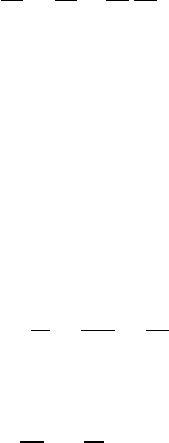
2.7 Shock waves and the Rankine–Hugoniot conditions 27
u
x
(a)
(b)
(c)
t = 0
t = t
B
t > t
B
Figure 2.2 The solution of (2.7)atdifferent times.
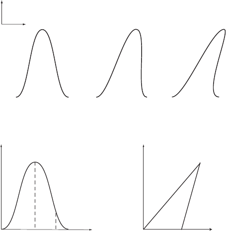
u
x
(a)
ξ = 0
ξ = x
I
x
I
x
x = 0
(b)
t
x = f(ξ)t + ξ
Figure 2.3 (a) A typical function u(ξ, 0) = f (ξ). (b) Characteristics associ-
ated with points ξ = 0, ξ = x
I
that intersect at t = t
B
. The point x
I
is the
inflection point of f (ξ).
In Figure 2.2 is shown a typical case and we can formally find the solu-
tion for values t > t
B
ignoring the singularities and triple-valued solution.
The value of time t, when characteristics first intersect, is denoted by t
B
–see
Figure 2.3.
2.7 Shock waves and the Rankine–Hugoniot conditions
Often we wish to take the solution further in time, beyond t = t
B
, but do not
want the multi-valued solution for physical or mathematical reasons. In many
important cases the solution has a nearly discontinuous structure. This is shown
schematically in Figure 2.4. Such a situation occurs in the case of the so-called
viscous Burgers equation
u
t
+ uu
x
= νu
xx
(2.9)
where ν is a constant; in this case there is a rapidly changing solution that
can be viewed as an approximation to a discontinuous solution for small
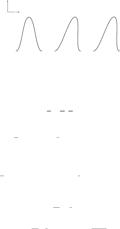
28 Linear and nonlinear wave equations
u
x
(a)
(b)
(c)
t = 0
t = t
B
t > t
B
Figure 2.4 Evolution of the solution to (2.7) with a “shock wave”.
ν (0 <ν 1). One way of introducing discontinuities, i.e., shocks, without
resorting to adding a “viscous” term (i.e., we keep ν = 0) is to consider (2.7)as
coming from a conservation law and its corresponding integral form. In other
words, (2.7) can be written in conservation law form as
∂
∂t
u +
∂
∂x
u
2
2
= 0
which in turn can be derived from the integral form
d
dt
x+Δx
x
u(x, t) dx +
1
2
u
2
(x +Δx, t) − u
2
(x, t)
= 0, (2.10)
in the limit Δx → 0. Equation (2.10) can support a shock wave since it is an
integral relation. Suppose between two points x
1
and x
2
we have a discontinuity
that can change in time x = x
s
(t) – see Figure 2.5. Then (2.10) reads
d
dt
x
s
(t)
x
1
u(x, t) dx +
x
2
x
s
(t)
u(x, t) dx
+
1
2
u
2
(x
2
, t) −u
2
(x
1
, t)
= 0.
Letting x
2
= x
s
(t) + , x
1
= x
s
(t) − , and >0, then as → 0, we have
x
2
→ x
+
and x
1
→ x
−
and so
(u(x
−
, t) −u(x
+
, t))
dx
s
dt
= −
1
2
u
2
(x
+
, t) −u
2
(x
−
, t)
and find
v
s
=
dx
s
dt
=
1
2
(
u(x
+
, t) −u(x
−
, t)
)
=
u
+
+ u
−
2
, (2.11)
where u
±
= u(x
±
, t). The last equation, (2.11), describes the speed of the shock,
v
s
= dx
s
/dt, in terms of the jump discontinuities.
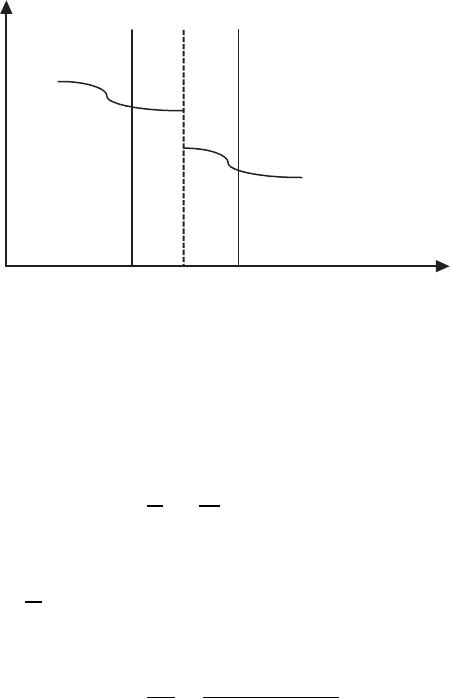
2.7 Shock waves and the Rankine–Hugoniot conditions 29
u(x,t)
x
x
1
x
2
x
s
Figure 2.5 A discontinuity in u(x, t)atx = x
s
(t).
We note that if (2.7) is generalized to
u
t
+ c(u)u
x
= 0,
the corresponding conservation law is
∂
∂t
u +
∂
∂x
(q(u)) = 0, (2.12)
where q
(u) = c(u), and its integral form is
d
dt
x+Δx
x
u(x, t) dx + q(u(x +Δx)) − q(u(x, t)) = 0.
Then following the same procedure as above, we find that the shock speed is
v
s
=
dx
s
dt
=
q(x
+
, t) −q(x
−
, t)
u
+
− u
−
. (2.13)
We note that in the limit x
+
→ x
−
we have v
s
→ q
(x
+
).
Equations (2.11) and (2.13) are sometimes referred to as the Rankine–
Hugoniot (RH) relations that were originally derived for the Euler equations
of fluid dynamics, cf. Lax (1987) and LeVeque (2002).
The RH relations, sometimes referred to as shock conditions, are used to
avoid multi-valued behavior in the solution, which would otherwise occur after
characteristics cross – see Figure 2.6. In order to make the problem well-posed
one needs to add admissibility conditions, sometimes called entropy-satisfying
conditions, to the relation. In their simplest form these conditions indicate
characteristics should be going into a shock as time increases, rather than
emanating, as that would be unstable, see Lax (1987) and LeVeque (2002).
30 Linear and nonlinear wave equations
t
x
t
B
x
−
(t)
x
+
(t)
v
s
=
d
x
s
/dt
Figure 2.6 Typical characteristic diagram.
Another viewpoint is that an admissibility relation should be the limit of, for
example, a viscous solution to Burgers’ equation, see (2.9), where the admis-
sible solution u
A
(x, t) = lim
ν→0
u(x, t; ν). We discuss Burgers’ equation in detail
later.
Let us consider the problem of fitting the discontinuities satisfying the shock
conditions into the smooth part of the solution, e.g., for x → x
+
(t), x → x
−
(t).
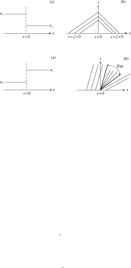
For example, consider (2.7) with the following initial condition:
u(x, 0) =
$
u
+
, x > 0
u
−
, x < 0.
where u
±
are constants. In the case where u
+
< u
−
, we see that the
characteristics cross immediately; i.e., they satisfy dx/dt = u,so
x = u
+
t + ξ, ξ > 0,
x = u
−
t + ξ, ξ < 0,
as indicated in Figure 2.7. The speed of the shock is given by
v
s
=
dx
dt
=
u
+
+ u
−
2
.
If u
+
= −u
−
the shock is stationary.
2.7 Shock waves and the Rankine–Hugoniot conditions 31
Figure 2.7 (a) Shock wave u
+
> u
−
. (b) Characteristics cross.
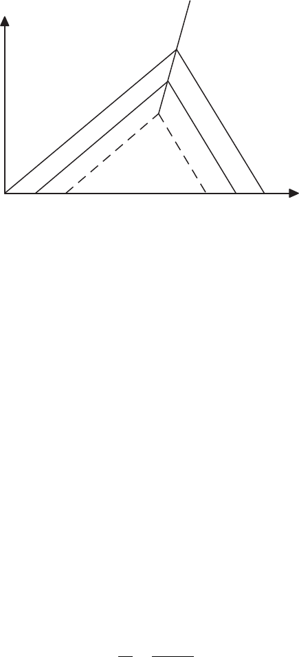
Figure 2.8 (a) “Rarefaction wave” u
+
< u
−
. (b) Characteristics do not cross.
There is a “fan” at x = 0.
On the other hand, if u
+
< u
−
, as in Figure 2.8, then the discontinuities do
not cross. In this case
x = u
+
t + ξ, ξ > 0,
x = u
−
t + ξ, ξ < 0,
x = ut,ξ= 0,
and the solution is termed a rarefaction wave with a fan at ξ = 0, u = x/t where
u
−
< x/t < u
+
.
Next we return briefly to discuss the viscous Burgers equation (2.9). If we
look for a traveling solution u = u(ζ), ζ = x−Vt−x
0
, where V, x
0
are constants,
and V the velocity of the (viscous shock) traveling wave, then
−Vu
ζ
+ uu
ζ
= νu
ζζ
.
Integrating yields
− Vu +
1
2
u
2
+ A = νu
ζ
, (2.14)
where A is the constant of integration. Further, if u → u
±
as x →±∞, where
u
±
are constants, then
A = −
1
2
u
2
±
− Vu
±
32 Linear and nonlinear wave equations
and by eliminating the constant A, we find
V =
1
2
u
2
+
− u
2
−
u
+
− u
−
=
1
2
(u
+
+ u
−
),
which is the same as the shock wave speed found earlier for the inviscid
Burgers equation. Indeed, if we replace Burgers’ equation by the generalization
u
t
+ (q(u))
x
= νu
xx
,
then the corresponding traveling wave u = u(ζ) would have its speed satisfy
V =
q(u
+
) − q(u
−
)
u
+
− u
−
[by the same method as for (2.7)], which agrees with the shock wave veloc-
ity (2.13) associated with (2.12). For the Burgers equation we can give an
explicit expression for the solution u by carrying out the integration of (2.14)
dζ =
νdu
u
2
/2 − Vu + A
with A = −((1/2)u
2
+
− (1/2)(u
+
+ u
−
)u
+
) = (1/2)u
+
u
−
. This results in
u =
u
+
+ u
−
e
(u
+
−u
−
)ζ/(2ν)
1 + e
(u
+
−u
−
)ζ/(2ν)
=
u
+
+ u
−
2
+
u
−
− u
+
2
tanh
u
+
− u
−
4ν
ζ
,
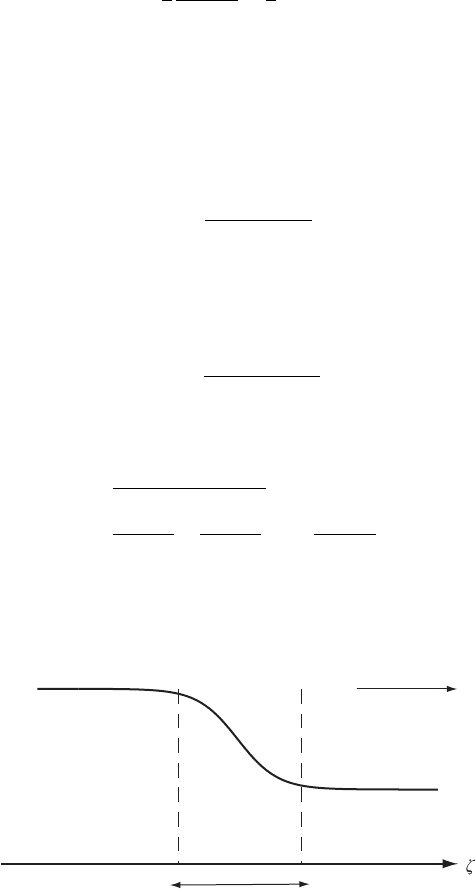
likeinFigure2.9.Thewidth of the viscous shock wave is proportional to
w = 4ν/(u
+
− u
−
).
u
−
u
+
w
V
Figure 2.9 Traveling viscous shock wave with velocity V and width
w = 4ν/(u
+
− u
−
).
2.8 Second-order equations: Vibrating string equation 33
2.8 Second-order equations: Vibrating string equation
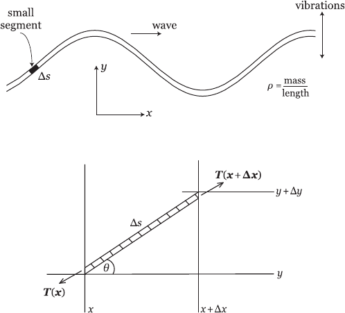
Let us turn our attention to deriving an approximate equation governing the
transverse vibration of a long string that is initially plucked and left to vibrate
(see Figure 2.10).
Let ρ be the mass density of the string: we assume it to be constant with ρ =
m/L, where m is the total mass of the string and L is its length. The string is in
equilibrium (i.e., at rest) when it is undisturbed along a straight line, which we
will choose to be the x-axis. When the string is plucked we can approximately
describe its vertical displacement from equilibrium at each point x as a function
y(x, t). Consider an infinitesimally small segment of the string, i.e., a segment
of length |Δs|1, where Δs
2
=Δx
2
+Δy
2
(see Figure 2.11). We will assume
no external forces and that horizontal acceleration is negligible. It follows from
Newton’s second law that
• difference in vertical tensions:
(T sin θ)|
x+Δx
− (T sin θ)|
x
=Δmy
tt
,
• difference in horizontal tensions:
(T cos θ)|
x+Δx
− (T cos θ)|
x
= 0.
Figure 2.10 Vibrations of a long string.
Figure 2.11 Tension forces acting on a small segment of the string.
34 Linear and nonlinear wave equations
In the limit |Δx|→0weassumethaty = y(x, t); then one has (in that limit)
sin θ =
Δy
Δs
=
Δy
(Δx)
2
+ (Δy)
2
→
y
x
1 + y
2
x
,
cos θ =
Δx
Δs
→
1
1 + y
2
x
.
Hence with these assumptions, in this limit, and using dm = ρds, Newton’s
equations become
ρ
ds
dx
y
tt
−
∂
∂x
T
y
x
1 + y
2
x
= 0,
∂
∂x
T
1
1 + y
2
x
= 0.
From the second equation we get that T = T
0
1 + y
2
x
, T
0
constant and, using
ds/dx =
1 + y
2
x
, the first equation yields
y
tt
=
T
0
ρ
1 + y
2
x
y
xx
. (2.15)
This is a nonlinear equation governing the vibrations of the string. If we
consider small-amplitude vibrations (i.e., |y
x
|1) and so neglect y
2
x
in the
denominator of the right-hand side we obtain, as an approximation, the linear
wave equation,
y
tt
− c
2
y
xx
= 0,
where c
2
= T
0
/ρ is the wave speed (speed of sound). However, we can approx-
imate (2.15) by assuming that |y
x
| is small but without neglecting it completely.
That can be done by taking the first correction term from a Taylor series of the
denominator:
1
1 + y
2
x
≈
1
1 + y
2
x
/2
≈ 1 −
1
2
y
2
x
.
Doing so leads to the nonlinear equation
y
tt
= c
2
y
xx
1 −
1
2
y
2
x
,
which is more amenable to analysis than (2.15), but still retains some of its
nonlinearity. It is interesting that this equation is a cubic nonlinear version
of (1.2) when ε h
2
/12. Note: if y
x
becomes large (e.g., a “shock” is formed),
then we need to go back to (2.15) and reconsider our assumptions.