Ablowitz M.A. Nonlinear Dispersive Waves: Asymptotic Analysis and Solitons
Подождите немного. Документ загружается.


10.4 Multiple-scale analysis of DM 285
where
−
∞
−∞
denotes the Cauchy principal value integral. Thus we have
R(t
1
, t
2
) =
iπ
2is (2π)
2
∞
−∞
e
iu
1
u
1
sgn
u
1
γ
+ 1
− sgn
1 −
u
1
γ
du
1
=
1
(4πs) · 2
−
∞
−γ
e
iu
1
u
1
du
1
−
−
−γ
−∞
e
iu
1
u
1
du
1
−
−
γ
−∞
e
iu
1
u
1
du
1
−
−
∞
γ
e
iu
1
u
1
du
1
=
1
(4πs) · 2
−
−
−γ
−∞
e
−iu
1
u
1
du
1
−
−
−γ
−∞
e
iu
1
u
1
du
1
+
−
∞
γ
e
iu
1
u
1
du
1
+
−
∞
γ
e
−iu
1
u
1
du
1
=
1
4πs
∞
γ
cos u
1
u
1
du
1
−
−γ
−∞
cos u
1
u
1
du
1
=
1
2πs
∞
γ
cos u
1
u
1
du
1
=
1
2πs
∞
1
cos γy
y
dy ≡
1
2πs
C
i
|t
1
t
2
|
s
.
where we used γ =
#
#
#
#
#
t
1
t
2
s
#
#
#
#
#
.
10.4.3 Dispersion-managed solitons
DM solitons are stationary solutions of the DMNLS equation, (10.30). We now
look for solutions of the form
ˆ
U(ω, Z) = e
iλ
2
Z/2
ˆ
F(ω),
where the only z-dependence is a linearly evolving phase. With this substitu-
tion, (10.30) becomes
λ
2
+
d
ω
2
2
ˆ
F(ω) −
∞
−∞
∞
−∞
r(ω
1
ω
2
)
ˆ
F(ω + ω
1
)
×
ˆ
F(ω + ω
2
)
ˆ
F
∗
(ω + ω
1
+ ω
2
) dω
1
dω
2
= 0
or
ˆ
F(ω) = −
2
λ
2
+
d
ω
2
∞
−∞
∞
−∞
r(ω
1
ω
2
)
ˆ
F(ω + ω
1
)
×
ˆ
F(ω + ω
2
)
ˆ
F
∗
(ω + ω
1
+ ω
2
) dω
1
dω
2
. (10.36)

286 Communications
Thus we wish to find fixed points of the integral equation (10.36). When r(x)is
not constant, obtaining closed-form solutions of this nonlinear integral equa-
tion is difficult. However we can readily obtain numerical solutions for
d
> 0.
Ablowitz and Biondini (1998) obtained numerical solutions using a fixed point
iteration technique similar to that originally introduced by Petviashvili (1976).
Below we first discuss a modification of this method called spectral renormal-
ization, which has proven to be useful in a variety of nonlinear problems where
obtaining localized solutions are of interest.
As we discussed earlier, another formulation of the non-local term is
∞
−∞
∞
−∞
r(ω
1
ω
2
)
ˆ
F(ω + ω
1
)
ˆ
F(ω + ω
2
)
ˆ
F
∗
(ω + ω
1
+ ω
2
) dω
1
dω
2
=
=
C
g(z)F
|
u
0
|
2
u
0
e
iω
2
C(ζ)/2
− iλ
2
Z/2
D
which is useful in the numerical schemes mentioned below. It should also be
noted from the multiple-scales perturbation expansion, that u
0
is obtained by
the inverse Fourier transform of
ˆu
0
(ω, ζ, Z) = F(ω)e
iλ
2
Z/2
e
−iω
2
C(ζ)/2
.
The naive iteration procedure is given by
ˆ
F
(m+1)
(ω) =
2
λ
2
+
d
ω
2
E
g(z)F
|
u
0
|
2
u
0
(m)
e
iω
2
C(ζ)/2−iλ
2
Z/2
F
≡ Im[
ˆ
F],
(10.37)
where m = 0, 1, 2,... and ˆu
(m)
0
=
ˆ
F
m
(ω)e
−iω
2
C(ζ)/2
.Atm = 0,
ˆ
F
(0)
(ω)istaken
to be the inverse Fourier transform of a Gaussian or “sech”-type function.
However, if we iterate (10.37) directly, the iteration generally diverges so we
renormalize as follows.
In (10.37) we substitute
ˆ
F = μ
ˆ
G. We then find the following iteration
equations
ˆ
G
n+1
= μ
2
n
I[
ˆ
G
n
]
with
μ
2
n
=
(
ˆ
G
n
,
ˆ
G
n
)
(
ˆ
G
n
, I[
ˆ
G
n
])
where (G
n
, I
n
) ≡
ˆ
G
∗
n
, I
n
dω and G
0
(t) can be a localized function, i.e., Gaus-
sian or sech profile. In either case, the iterations converge rapidly. More details
can be found in Ablowitz and Musslimani (2005) and Ablowitz and Horikis
(2009a).
10.4 Multiple-scale analysis of DM 287
−5
0
5
0
0.5
1
0
2
4
Time t
Distance ζ
Amplitude U
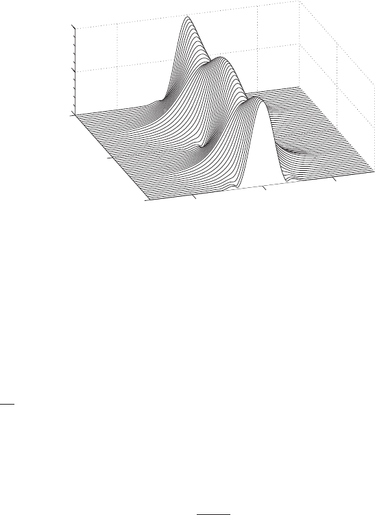
Figure 10.6 Fast evolution, u(z, t), of the stationary solitons of DMNLS,
reconstructed from the perturbation expansion, with
d
= 1, s = 1andλ = 4.
In Figure 10.6 a typical DM soliton is represented in physical space
(u ∼u
(0)
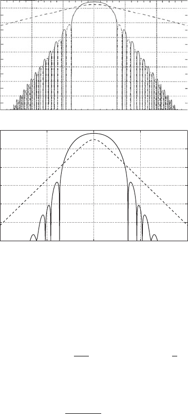
(z, t)). Figure 10.7 compares typical DM solitons in the Fourier and
temporal domains in logarithmic scales. The dashed line is a classical soliton
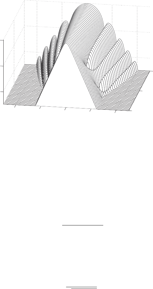
with the same FWHM. Figure 10.8 depicts a class of DM solitons for vary-
ing values of the map strength, s. In the figures note that u(z, t) ∼ u
(0)
. Hence
from ˆu
(0)
(ω) =
ˆ
U(ω, Z)e
−iC(ζ)ω
2
/2
, with
ˆ
U(ω, Z) = F(ω)e
iλ
2
Z/2
, then u
(0)
(t) =
1
2π
∞
−∞
ˆu
(0)
(ω)e
iωt
dω. The latter yields the behavior in physical space.
Originally these methods where introduced by Petviashvili (1976) to find
solutions of the KP equations. In the context of DMNLS theory (see Ablowitz
et al., 2000b; Ablowitz and Musslimani, 2003) the following implementation
of Petviashvili’s method is employed
ˆ
F(ω) =
S
L
[
ˆ
F]
S
R
[
ˆ
F]
p
K[
ˆ
F],
where
S
L
=
∞
−∞
#
#
#
ˆ
F
#
#
#
2
dω,
S
R
=
∞
−∞
ˆ
F
∗
· K[
ˆ
F] dω
and
K[
ˆ
F] ≡
∞
−∞
∞
−∞
r(ω
1
ω
2
)
ˆ
F(ω + ω
1
)
ˆ
F(ω + ω
2
)
ˆ
F
∗
(ω + ω
1
+ ω
2
) dω
1
dω
2
.
288 Communications
10
0
10
–2
10
–4
10
–6
Amplitude |F(ω)|
10
–8
10
–10
10
–12
10
–14
–15 –10 –5 0
Frequency
ω
51015
−10 −5 0 5 10
−5
−4
−3
−2
−1
0
1
Frequency
Amplitude Log[
ˆ
f (ω)]
ω
Figure 10.7 Shape of the stationary pulses in the Fourier and temporal
domains for s = 1andλ = 4.
The power p is usually chosen such that the degree of homogeneity of the
right-hand side is zero, i.e.,
deg{homog.}(RHS) =
ˆ
F
2p
ˆ
F
4p
ˆ
F
3
=
ˆ
F
3−2p
⇒ p =
3
2
.
With this choice for p, we employ the iteration scheme
ˆ
F
(m+1)
(ω) =
S
L
[
ˆ
F
(m)
]
S
R
[
ˆ
F
(m)
]
3/2
K[
ˆ
F
(m)
]. (10.38)
Adifficulty with this “homogeneity” method is how to handle more complex
nonlinearities that do not have a fixed nonlinearity, such as mixed nonlinear
terms with polynomial nonlinearity, or more complex nonlinearities, such as
saturable nonlinearity u/(1 + |u|
2
) or transcendental nonlinearities.
We further note:
• DM solitons are well approximated by a Gaussian,
ˆ
F(ω) ae
−bω
2
/2
,fora
wide range of s and λ.
10.4 Multiple-scale analysis of DM 289
−20
−10
0
10
20
0
8
16
−4
−2
0
Map
Strength s
Time t
Amplitude Log[f(t)]
Figure 10.8 Shape of the stationary pulses in the temporal domain for λ = 1
and various values of s.
• The parameters a and b are dependent upon s and λ, a = a(s,λ), b =
b(s,λ).
• For s 1, |
ˆ
F| grows |
ˆ
F|(ω) ∼ s
1/2
.
See also Lushnikov (2001).
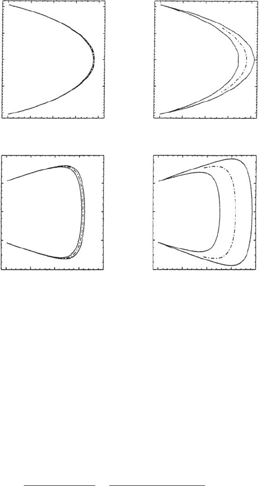
Figure 10.9 shows “chirp” versus amplitude phase plane plots for four differ-
ent DM soliton systems. This figure shows how the multi-scale approximation
improves as z
a
= ε → 0. Here the chirp is calculated as
c(z) =
∞
−∞
t Im
{
u
∗
u
t
}
dt
∞
−∞
t
2
|
u
|
2
dt
, (10.39)
where Im(x) represents the imaginary part of x. If we approximate the DMNLS
solution as a Gaussian exponential, then
ˆ
U
DMNLS
= ae
−bω
2
/2
e
−iC(ζ)ω
2
/2
,
so that in the time domain, u(t) =
a
√
2π(b + iC)
e
−t
2
/2(b+iC)
, then the chirp c(z)
is found to be given by c(z) = C(ζ) = C(z/z
a
); that is also given by (10.39)
after integration.
290 Communications
0.2
0.1
0.0
–0.1
–0.2
0.90
2.5
–0.4
–0.2
0.0
Chirp, c(z) Chirp, c(z)
0.2
0.1
0.0
–0.1
–0.2
Chirp, c(z)
0.2
0.4
(c)
–0.4
–0.2
0.0
Chirp, c(z)
0.2
0.4
(d)
(a) (b)
3.0 3.5 4.0 4.5
0.92 0.94 0.96 0.98
Peak amplitude, |q|
max
(z)
0.90 0.92 0.94 0.96 0.98
Peak amplitude, |q|
max
(z)
Peak amplitude, |q|
max
(z)
2.5 3.0 3.5 4.0 4.5
Peak amplitude, |q|
max
(z)
Figure 10.9 The periodic evolution of the pulse parameters: chirp c(z)versus
the peak amplitude. The dot–dashed line represents the leading-order approx-
imation, u
0
(ζ,t), as reconstructed from the DMNLS pulses and (10.26); the
solid lines represent numerical solitions of the PNLS equation (10.19) with
g = 1 and the same pulse energy. The four cases correspond to: (a) s = 1,
λ = 1, z
a
= 0.02; (b) s = 1, λ = 1, z
a
= 0.2; (c) s = 4, λ = 4, z
a
= 0.02;
(d) s = 4, λ = 4, z
a
= 0.2. The pulse energies are
f
2
= 2.27 for cases
(a) and (b), and
f
2
= 38.9 for cases (c) and (d). See also Ablowitz et al.
(2000b).
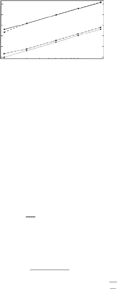
In Figure 10.10 we plot the relative L
2
norm of the difference between the
stationary soliton solution of the DMNLS and the numerical solution of the
original perturbed (PNLS) equation (10.19); equations with the same energy,
sampled at the mid-point of the fiber segment. The difference is normalized to
the L
2
-norm of the numerical solution of the PNLS equation; that is
f
DMNLS
− f
PNLS
2
2
f
PNLS
=
∞
−∞
dt
|
f
DMNLS
− f
PNLS
|
2
∞
−∞
dt
|
f
PNLS
|
2
.
10.4 Multiple-scale analysis of DM 291
10
–2
10
–3
10
–4
10
–5
10
–6
||f
DMNLS
–f
PNLS
||
2
/||f
PNLS
||
2
10
–7
10
–3
10
–2
Z
a
Figure 10.10 Comparison between stationary solutions of the DMNLS equa-
tion f (t) and the solutions u(z, t) of the PNLS equation (10.19) with the same
energy taken at the mid-point of the anomalous fiber segment for g = 1,
d
= 1andfivedifferent values of z
a
: 0.01, 0.02, 0.05, 0.1 and 0.2. Solid
line: s = 4, λ = 4,
f
2
= 38.9; dashed line: s = 1, λ = 4,
f
2
= 20.7; dot–
dashed line: s = 4, λ = 1,
f
2
= 3.1; dotted line: s = 1, λ = 1,
f
2
= 2.27.
See also (Ablowitz et al., 2000b).
We also note there is an existence proof of DMNLS soliton solutions as
ground states of a Hamiltonian. Furthermore, it can be proven that the DMNLS
equation (10.30) is asymptotic, i.e., its solution remains close to the solution
of the original NLS equation (10.21), see Zharnitsky et al. (2000).
10.4.4 Numerical “averaging” method
To find soliton solutions from the original PNLS equation (10.19) we may use
a numerical averaging method (Nijhof et al., 1997, 2002). In this method one
starts with the non-dimensional PNLS equation, (10.19):
iu
z
+
d(z)
2
u
tt
+ g|u|
2
u = 0,
and an initial guess for the DM soliton, e.g., a Gaussian, u
g
(z = 0, t) = u
g
(t) =
u
(0)
with E
0
=
∞
−∞
#
#
#
u
g
#
#
#
2
dt. Next, numerically integrate from z = 0toz = z
a
to get u(z = z
a
, t); call this ˜u(t) =
|
u(t)
|
e
iθ(t)
. Then one takes the following
“average”:
˜
˜u(t) =
u
g
(t) + ˜u(t)e
−iθ(0)
2
.
Then u
(1)
is obtained by renormalizing the energy: u
(1)
=
˜
˜u(t)
'
E
0
˜
˜
E
, where
˜
˜
E =
∞
−∞
#
#
#
˜
˜u
2
#
#
#
dt. This procedure is repeated until u
(m)
(t) converges. This method

292 Communications
can also be used to obtain the DM soliton solutions of the PNLS equation and
the solid line curves in Figure 10.9.
10.4.5 The higher-order DMNLS equation
The analysis of Section 10.4 can be taken to the next order in z
a
(Ablowitz
et al., 2002b). In the Fourier domain we write the more general DMNLS
equation in the form
i
ˆ
U
z
−
d
2
ω
2
ˆ
U
+
n
0
(ω,z)
8967
∞
−∞
∞
−∞
dω
1
dω
2
ˆ
U(ω + ω
1
)
ˆ
U(ω + ω
2
)
ˆ
U
∗
(ω + ω
1
+ ω
2
)r(ω
1
ω
2
)
=z
a
ˆn
1
(ω, z) + ···.
The method is similar to those described earlier for water waves and nonlinear
optics. We find ˆn
1
such that the secular terms at higher order are removed.
Recalling u = u
0
+ u
1
+
2
u
2
+ ··· where = z
a
, we substitute this into
the perturbed NLSE equation (10.21), and as before employ multiple scales.
We find
O
−1
: Lu
0
= i
∂u
0
∂ζ
+
Δ(z)
2
∂
2
u
0
∂t
2
= 0
O
(
1
)
: Lu
1
= −
i
∂u
0
∂Z
+
d
2
∂u
0
∂t
2
+ g(ζ)
|
u
0
|
2
u
0
O
(
)
: Lu
2
= −
i
∂u
1
∂Z
+
d
2
∂u
1
∂t
2
+ g(ζ)
2
|
u
0
|
2
u
1
+ u
2
0
u
∗
1
.
The first two terms are the same as what we found earlier for the DMNLS
equation. At O
−1
,
u
0
=
ˆ
U(ω, Z)e
−iω
2
C(ζ)/2
, C(ζ) =
ζ
0
Δ(ζ
) dζ
,
and at O
(
1
)
i
∂ˆu
1
∂ζ
−
Δ(ζ)
2
ω
2
ˆu
1
= −
i
∂ˆu
0
∂Z
−
d
2
ω
2
ˆu
0
+ g(ζ)F
|
u
0
|
2
u
0
= −
i
∂
ˆ
U
∂Z
− ω
2
d
2
ˆ
U
e
−iω
2
C(ζ)/2
− gF
|
u
0
|
2
u
0
.

10.4 Multiple-scale analysis of DM 293
Thus,
∂
∂ζ
iˆu
1
e
iC(ζ)ω
2
/2
= −
i
∂
ˆ
U
∂Z
− ω
2
d
2
ˆ
U
− g(ζ)e
iC(ζ)ω
2
/2
F
|
u
0
|
2
u
0
≡
ˆ
F
1
.
To remove secular terms we enforce periodicity of the right-hand side, i.e., we
require
C
ˆ
F
1
D
= 0, where
C
ˆ
F
1
D
=
1
0
ˆ
F
1
dζ. This implies
i
∂
ˆ
U
∂Z
− ω
2
d
2
ˆ
U + ˆn
0
(ω, Z) = 0,
with
ˆn
0
(ω, Z) =
C
g(ζ)e
iω
2
C(ζ)/2
F
|
u
0
|
2
u
0
D
.
This is the DMNLS equation (10.25) that can be transformed to (10.30).
We now take
i
∂
ˆ
U
∂Z
− ω
2
d
2
ˆ
U + ˆn
0
(ω, Z) = ˆn
1
(ω, Z) + ···. (10.40)
Once we obtain ˆn
1
(ω, Z) then (10.40) will be the higher-order DMNLS equa-
tion. However we need to solve for u
1
since it will enter into the calculation for
n
1
. Using an integrating factor in the O(1) equation, adding and subtracting a
mean term and using the DMNLS equation, we find
∂
∂ζ
iˆu
1
e
iC(ζ)ω
2
/2
= −
i
∂U
∂Z
− ω
2
d
2
U
+
C
g(ζ)e
iω
2
C(ζ)/2
F
|
u
0
|
2
u
0
D
− g(ζ)e
iω
2
C(ζ)/2
F
|
u
0
|
2
u
0
+
C
g(ζ)e
iω
2
C(ζ)/2
F
|
u
0
|
2
u
0
D
iˆu
1
e
iC(ζ)ω
2
/2
= −
ζ
0
g(ζ)e
iω
2
C(ζ)/2
F
|
u
0
|
2
u
0
dζ
+ ζ
C
g(ζ)e
iω
2
C(ζ)/2
F
|
u
0
|
2
u
0
D
+
ˆ
U
1H
(ω, Z).
Therefore,
ˆu
1
e
iC(ζ)ω
2
/2
=i
ζ
0
g(ζ)e
iω
2
C(ζ)/2
F
|
u
0
|
2
u
0
dζ
− iζ
C
g(ζ)e
iω
2
C(ζ)/2
F
|
u
0
|
2
u
0
D
− i
ˆ
U
1H
(ω, Z),

294 Communications
where
ˆ
U
1H
(ω, Z) is an integration “constant” to be determined. We choose
U
1
(ω, Z) such that
C
u
1
(ω, Z)e
iC(ζ)ω
2
/2
D
=
1
0
u
1
e
iC(ζ)ω
2
/2
dζ = 0. This is done
to ensure that u
1
does not produce secular terms at next order. Therefore
ˆ
U
1H
=
G
ζ
0
g(ζ
)e
iω
2
C(ζ
)/2
F
|
u
0
|
2
u
0
dζ
H
−
1
2
C
g(ζ)e
iω
2
C(ζ)/2
F
|
u
0
|
2
u
0
D
.
This fixes ˆu
1
and thus u
1
. Then u
2
is given by
∂
∂ζ
iˆu
2
e
iC(ζ)ω
2
/2
= −
$
ˆn
1
(ω, Z) + e
iC(ζ)ω
2
/2
i
∂ˆu
1
∂Z
−
−
d
2
ω
2
ˆu
1
+ g(ζ)
ˆ
P
1
(ζ,Z,ω)
2
≡
ˆ
F
2
,
where
ˆ
P
1
= F
2
|
u
0
|
2
u
1
+ u
2
0
u
∗
1
. To eliminate secularities we require
C
ˆ
F
2
D
= 0. This condition determines ˆn
1
and we obtain the higher-order
DMNLS equation. Thus, since
C
ˆu
1
e
iC(ζ)ω
2
/2
D
= 0, we have
ˆn
1
= −
C
g(ζ)e
iω
2
C(ζ)/2
ˆ
P
1
(ω, Z)
D
. (10.41)
With ˆn
0
and ˆn
1
we now have the higher-order DMNLS equation (10.40). The
form (10.41) is useful numerically. But as with the standard DMNLS theory
we also note that we can write ˆn
1
as a multiple integral in the Fourier domain.
After manipulation we find,
ˆn
1
=
−i
(2π)
4
∞
−∞
∞
−∞
∞
−∞
∞
−∞
dω
1
dω
2
dΩ
1
dΩ
2
r
1
(ω
1
ω
2
, Ω
1
Ω
2
)
2
ˆ
U(ω + ω
1
) ×
ˆ
U
∗
(ω + ω
1
+ ω
2
)
ˆ
U(ω + ω
2
+Ω
1
)
ˆ
U(ω + ω
2
+Ω
2
)
×
ˆ
U
∗
(ω + ω
2
+Ω
1
+Ω
2
) −
ˆ
U(ω + ω
1
)
ˆ
U(ω + ω
2
)
ˆ
U
∗
(ω + ω
1
+ ω
2
+Ω
1
)
×
ˆ
U(ω + ω
1
+ ω
2
− Ω
2
)
ˆ
U(ω + ω
1
+ ω
2
+Ω
1
− Ω
2
)
,
(10.42)
where the kernel is given by
r
1
(x, y) =
G
g(ζ)K(ζ, x)
ζ
0
g(ζ
)K(ζ
, y) dζ
H
−
g(ζ)K(ζ, x)
G
ζ
0
g(ζ
)K(ζ
, y) dζ
H
−
C
(ζ −
1
2
)g(ζ)K(ζ, x)
D
g(ζ)K(ζ,y)
,