Ablowitz M.A. Nonlinear Dispersive Waves: Asymptotic Analysis and Solitons
Подождите немного. Документ загружается.

10.3 Dispersion-management 275
where we note that now k
is a function of z and for simplicity we omit
gain and loss for now. For classical solitons the dispersive coefficient, k
,is
constant. However, with dispersion-management the dispersion varies with z
and thus k
= k
(z). To normalize this equation (see also Section 10.1.1)
we take A =
√
P
∗
u, z = z
∗
z
and t = t
∗
t
; recall the nonlinear distance is
given by z
∗
= 1/νP
∗
and t
∗
is determined by the FWHM of the pulse, t
FWHM
.
Then (10.18) becomes
iu
z
+
(−k
(z))
2
z
∗
t
2
∗
u
tt
+ νP
∗
z
∗
|u|
2
u = 0.
Taking k
∗
= t
2
∗
/z
∗
we get
iu
z
+
3
−k
(z)/k
∗
4
2
u
tt
+ |u|
2
u = 0.
The dispersion d(z) = −k
(z)/k
∗
is dependent on z and can be written as
an average plus a varying part, k
=
k
+ δk
(z), where
k
represents the
average and is given by
k
=
k
1
1
+ k
2
2
/ where
1
and
2
are the lengths
of the anomalous and normal dispersion segments, respectively, and =
1
+
2
,
and usually l = l
a
(l
a
: the length between amplifiers). The non-dimensionalized
dispersion is given by k
/k
∗
=
d
+
˜
Δ(z) = d(z), with the average dispersion
denoted by
d
=
k
/k
∗
and the varying part around the average:
˜
Δ(z) =
δk
/k
∗
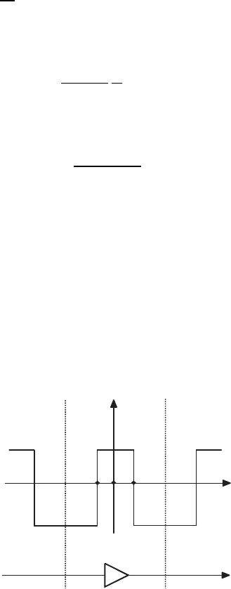
. Typically it is taken to be a piecewise constant function as illustrated in
Figure 10.5.
Δ(z)
θ/2
amplifier
0
z/z
a
−θ/2
Δ
2
Δ
1
Figure 10.5 A schematic diagram of a two-fiber dispersion-managed cell.
Typically the periodicity of the dispersion-management is equal to the
amplifier spacing, i.e., =
a
or in normalized form, z
a
= l
a
/z
∗
.

276 Communications
The non-dimensionalized NLS equation is now
iu
z
+
d(z)
2
u
tt
+ |u|
2
u = 0.
Damping and amplification can be added, as before, which leads to our
fundamental model:
iu
z
+
d(z)
2
u
tt
+ g(z)|u|
2
u = 0. (10.19)
If d(z) does not change sign, we can simplify (10.19) by letting
˜z(z) =
z
0
h(z
) dz
so that ∂
z
= h(z)∂
˜z
, where h(z) is to be determined. Equation (10.19) then
becomes
iu
˜z
+
1
2
d(z)
h(z)
u
tt
+
g(z)
h(z)
|u|
2
u = 0.
If fibers could be constructed so that h(z) = d(z) = g(z), then we would obtain
the classical NLS equation:
iu
˜z
+
1
2
u
tt
+ |u|
2
u = 0.
This type of fiber is called “dispersion following the loss profile”.
Unfortunately, it is very difficult to manufacture such fibers. An idea first
suggested in 1980 (Lin et al., 1980) that has become standard technology is
to fuse together fibers that have large and different, but (nearly) constant, dis-
persion characteristics. A two-step “dispersion-managed” transmission line is
modeled as follows:
d(z) =
d
+
Δ(z/z
a
)
z
a
,
Δ
=
1
0
Δ(ζ) dζ = 0,ζ=
z
z
a
.
We quantify the parameters of a two-step map as illustrated in Figure 10.5.The
variation of the dispersion is given by Δ(ζ),
Δ(ζ) =
⎧
⎪
⎪
⎨
⎪
⎪
⎩
Δ
1
, 0 ≤|ζ| <θ/2,
Δ
2
,θ/2 < |ζ| < 1/2.

10.4 Multiple-scale analysis of DM 277
In this two-step map we usually parameterize Δ
j
, j = 1, 2, by
Δ
1
=
2s
θ
, Δ
2
=
−2s
1 − θ
,
where
Δ
= 0 and s is termed the map strength parameter, defined as
s =
θΔ
1
− (1 − θ)Δ
2
4
=
area enclosed byΔ
4
. (10.20)
Note that
Δ
= θΔ
1
+ (1 − θ)Δ
2
= 0, as it should be by its definition.
Remarkably dispersion-management is also an important technology that is
used to produce ultra-short pulses in mode-locked lasers, such as in Ti:sapphire
lasers (Ablowitz et al., 2004a; Quraishi et al., 2005; Ablowitz et al., 2008)
discussed in the next chapter.
10.4 Multiple-scale analysis of DM
In this section we apply the method of multiple scales to (10.19) (see Ablowitz
and Biondini, 1998):
iu
z
+
1
2
d
+
Δ(ζ)
z
a
u
tt
+ g(ζ)|u|
2
u = 0. (10.21)
In (10.21), let us call our small parameter z
a
= ε, assume z
a
≡ 1,
and define u = u(t,ζ,Z; ), ζ = z/, and Z = z; hence,
∂
∂z
=
1
∂
∂ζ
+
∂
∂Z
.
Thus,
1
i
∂u
∂ζ
+
1
2
Δ(ζ)
∂
2
u
∂t
2
+ i
∂u
∂Z
+
1
2
d
∂
2
u
∂t
2
+ g(ζ)|u|
2
u = 0.
With a standard multiple-scales expansion u = u
0
+ u
1
+
2
u
2
+ ···,wehave
at leading order, O
(
1/
)
,
i
∂u
0
∂ζ
+
Δ(ζ)
2
∂
2
u
0
∂t
2
= 0. (10.22)
We solve (10.22) using Fourier transforms, defined by (inverse transform)
u
0
(t,ζ,Z) ≡
1
2π
∞
−∞
ˆu
0
(ω, ζ, Z)e
iωt
dω,
and (direct transform)
ˆu
0
(ω, ζ, Z) = F
{
u
0
}
≡
∞
−∞
u
0
(t,ζ,Z)e
−iωt
dt.

278 Communications
Taking the Fourier transform of (10.22) and solving the resulting ODE,
we find
∂ˆu
0
∂ζ
−
ω
2
2
Δ(ζ)ˆu
0
= 0, (10.23a)
ˆu
0
(ω, ζ, Z) =
ˆ
U(ω, Z)e
−iω
2
C(ζ)/2
, (10.23b)
where C(ζ) =
ζ
0
Δ(ζ
) dζ
is the integrated dispersion.
At the next order, O(1), we have
i
∂u
1
∂ζ
+
Δ(ζ)
2
∂
2
u
1
∂t
2
= F
1
, (10.24)
where
−F
1
≡ i
∂u
0
∂Z
+
1
2
d
∂
2
u
0
∂t
2
+ g(ζ)|u
0
|
2
u
0
.
Again using the Fourier transform, (10.24) becomes
iˆu
1ζ
−
ω
2
2
Δ(ζ)ˆu
1
=
(
F
1
,
or
i
∂
∂ζ
ˆu
1
e
iω
2
C(ζ)/2
=
(
F
1
e
iω
2
C(ζ)/2
.
Hence
iˆu
1
e
iω
2
C(ζ)/2
ζ
=ζ
ζ
=0
=
ζ
0
(
F
1
e
iω
2
C(ζ)/2
dζ.
Since C(ζ) is periodic in ζ and Δ has zero mean, ˆu
0
is also periodic in ζ. There-
fore to remove secular terms we must have
C
(
F
1
e
iω
2
C(ζ)/2
D
= 0. Thus we require
that
C
(
F
1
e
iω
2
C(ζ)/2
D
=
1
0
(
F
1
e
iω
2
C(ζ)/2
dζ = 0,
or
1
0
i
∂ˆu
0
∂Z
−
d
2
ω
2
ˆu
0
e
iω
2
C(ζ)/2
dζ
+
1
0
g(ζ)F
|u
0
|
2
u
0
e
iω
2
C(ζ)/2
dζ = 0.
Using (10.23b) we get the dispersion-managed NLS (DMNLS) equation:
i
∂
ˆ
U
∂Z
−
d
2
ω
2
ˆ
U +
C
g(ζ)F
|
u
0
|
2
u
0
e
iω
2
C(ζ)/2
D
= 0. (10.25)

10.4 Multiple-scale analysis of DM 279
10.4.1 The DMNLS equation in convolution form
Equation (10.25) is useful numerically, but analytically it is often better to
transform the nonlinear term to Fourier space. Using the Fourier transform
u
0
(t,ζ,Z) =
1
2π
∞
−∞
ˆ
U(ω, Z)e
−iω
2
C(ζ)/2
e
iωt
dω (10.26)
in the nonlinear term in (10.25), we find, after interchanging integrals (see
Section 10.4.2 for a detailed discussion):
C
g(ζ)F[
|
u
0
|
2
u
0
]e
iω
2
C(ζ)/2
D
=
∞
−∞
∞
−∞
r(ω
1
ω
2
)
ˆ
U(ω + ω
1
, z)
×
ˆ
U(ω + ω
2
, z)
ˆ
U
∗
(ω + ω
1
+ ω
2
, z) dω
1
dω
2
,
(10.27)
where
r(ω
1
ω
2
) =
1
(2π)
2
1
0
g(ζ)exp
%
iω
1
ω
2
C(ζ)
&
dζ. (10.28)
If g(z) = 1, i.e., the lossless case, we find for the two-step map, depicted in
Figure 10.5, that
r(x) =
sin sx
(2π)
2
sx
, (10.29)
where s is called the DM map strength [see (10.20)]. This leads to another
representation of the DMNLS equation in “convolution form”
i
ˆ
U
Z
−
d
2
ω
2
ˆ
U +
∞
−∞
∞
−∞
r(ω
1
ω
2
)
ˆ
U(ω + ω
1
, z)
ˆ
U(ω + ω
2
, z)
ˆ
U
∗
(ω + ω
1
+ ω
2
, z) dω
1
dω
2
= 0, (10.30)
where r(ω
1
ω
2
)isgivenin(10.28)(Ablowitz and Biondini, 1998; Gabitov and
Turitsyn, 1996).
The above DMNLS equation has a natural dual in the time domain. Tak-
ing the inverse Fourier transform of (10.30) yields (see Section 10.4.2 for
details)
iU
Z
+
d
2
U
tt
+
∞
−∞
∞
−∞
R(t
1
, t
2
)U(t
1
)U(t
2
)U
∗
(t
1
+ t
2
− t) dt
1
dt
2
= 0,
(10.31)

280 Communications
where
R(t
1
, t
2
) =
∞
−∞
∞
−∞
r(ω
1
ω
2
)e
iω
1
t
2
e
iω
2
t
1
dω
1
dω
2
.
Note that if Δ(z) → 0, we recover the classical NLS equation since it can
be shown that as s → 0, r → 1/(2π)
2
, R(t
1
, t
2
) → δ(t
1
)δ(t
2
), recalling that
δ(t) =
1
2π
e
iωt
dt. When g(z) = 1, the lossless case, we also find
R(t
1
, t
2
) =
1
2πs
Ci
|t
1
t
2
|
s
with
Ci(x) =
∞
x
cos u
u
du.
10.4.2 Detailed derivation
In this subsection we provide the details underlying the derivation of (10.27)
and (10.31) as well as the special cases of (10.29) when g = 1. We start by
writing (10.27) explicitly:
I(ω) = I ≡
C
g(ζ)F
|
u
0
|
2
u
0
e
iω
2
C(ζ)/2
D
=
1
0
g(ζ)
∞
−∞
dt
1
2π
∞
−∞
ˆ
U(ω
1
, Z)e
−iω
2
1
C(ζ)/2
e
iω
1
t
dω
1
×
1
2π
∞
−∞
ˆ
U(ω
2
, Z)e
−iω
2
2
C(ζ)/2
e
iω
2
t
dω
2
×
1
2π
∞
−∞
ˆ
U
∗
(ω
3
, Z)e
iω
2
3
C(ζ)/2
e
−iω
3
t
dω
3
× e
−iωt
e
iω
2
C(ζ)/2
dζ.
Interchanging the order of integration and grouping the exponentials together,
I =
1
0
g(ζ)
∞
−∞
∞
−∞
∞
−∞
1
2π
2
ˆ
U(ω
1
, Z)
ˆ
U(ω
2
, Z)
×
ˆ
U
∗
(ω
3
, Z)e
−i
(
ω
2
1
+ω
2
2
−ω
2
3
−ω
2
)
C(ζ)/2
×
1
2π
∞
−∞
e
i(ω
1
+ω
2
−ω
3
−ω)t
dt dω
1
dω
2
dω
3
dζ.
Recall that the Dirac delta function can be written as
δ(ω
− ω) =
1
2π
∞
−∞
e
i(ω
−ω)t
dt,

10.4 Multiple-scale analysis of DM 281
where ω
= ω
1
+ ω
2
− ω
3
. Thus, with ω
3
= ω
1
+ ω
2
− ω,
I =
1
0
g(ζ)
∞
−∞
∞
−∞
1
2π
2
ˆ
U(ω
1
, Z)
ˆ
U(ω
2
, Z)
ˆ
U
∗
(ω
1
+ ω
2
− ω, Z)
× exp
−i
(ω
1
+ ω
2
)ω − ω
1
ω
2
− ω
2
C(ζ)
dω
1
dω
2
dζ. (10.32)
A more symmetric form is obtained when we use
ω
1
= ω + ˜ω
1
ω
2
= ω + ˜ω
2
2
⇒ ω
1
+ ω
2
− ω = ˜ω
1
+ ˜ω
2
+ ω.
Note that −ω
1
ω
2
+ (ω
1
+ ω
2
)ω = − (ω + ˜ω
1
)(ω + ˜ω
2
) + (˜ω
1
+ ˜ω
2
+ ω)ω =
−˜ω
1
˜ω
2
. Equation (10.32) can now be written, after dropping the
tildes,
I =
1
0
g(ζ)
∞
−∞
∞
−∞
ˆ
U(ω
1
+ ω, Z)
ˆ
U(ω
2
+ ω, Z)
×
ˆ
U
∗
(ω
1
+ ω
2
+ ω, Z)
1
2π
2
e
iω
1
ω
2
C(ζ)
dω
1
dω
2
dζ. (10.33)
We now define the DMNLS kernel r:
r(x) ≡
1
(2π)
2
1
0
g(ζ)e
ixC(ζ)
dζ.
Then (10.33) becomes
I =
∞
−∞
∞
−∞
r(ω
1
ω
2
)
ˆ
U(ω
1
+ ω, Z)
×
ˆ
U(ω
2
+ ω, Z)
ˆ
U
∗
(ω
1
+ ω
2
+ ω, Z) dω
1
dω
2
,
which is the third term in (10.30), i.e., (10.27).
For the lossless case, i.e., g(ζ) = 1 and a two-step map, r(x), the analysis
can be considerably simplified. We now give details of this calculation. First,
for a two-step map with C(0) = 0
C(ζ) =
ζ
0
Δ(ζ
) dζ
=
⎧
⎪
⎪
⎪
⎪
⎪
⎨
⎪
⎪
⎪
⎪
⎪
⎩
Δ
1
ζ, 0 <ζ<θ/2
Δ
2
ζ + C
1
,θ/2 <ζ<1 − θ/2
Δ
1
ζ + C
2
, 1 − θ/2 <ζ<1
C
1
=Δ
1
θ/2 − Δ
2
θ/2 = (Δ
1
− Δ
2
)θ/2
C
2
= −Δ
1
,

282 Communications
where C
1,2
are obtained by requiring continuity at ζ = θ/2, 1−θ/2, respectively.
Recall that since
Δ
= 0, we have Δ
1
θ +Δ
2
(1 − θ) = 0. Thus,
I =
1
0
e
ixC(ζ)
dζ
=
θ/2
0
e
iΔ
1
ζx
dζ +
1−θ/2
θ/2
e
i(Δ
2
ζ+C
1
)x
dζ +
1
1−θ/2
e
i(Δ
1
ζ+C
2
)x
dζ
I =
e
iΔ
1
θx/2
− 1
iΔ
1
x
+ e
iC
1
x
e
iΔ
2
(1−θ/2)x
− e
iΔ
2
θx/2
iΔ
2
x
+ e
iC
2
x
e
iΔ
1
x
− e
iΔ
1
(1−θ/2)x
iΔ
1
x
.
Using C
1
= (Δ
1
− Δ
2
)θ/2 and C
2
+Δ
1
= 0,
I =
e
iΔ
1
θx/2
−e
−iΔ
1
θ/2
iΔ
1
x
+
e
i(Δ
2
(1−θ/2)x+(Δ
1
−Δ
2
)θ/2)
−e
i(Δ
2
θx/2+(Δ
1
−Δ
2
)θ/2)
iΔ
2
x
I =
e
iΔ
1
(θ/2)x
− e
−iΔ
1
(θ/2)x
iΔ
1
x
+
e
iΔ
2
(1−θ)x+Δ
1
θ/2
− e
−iΔ
1
(θ/2)x
iΔ
2
x
.
Then using Δ
2
(1 − θ) = −Δ
1
θ, we get
I =
e
iΔ
1
(θ/2)x
− e
−iΔ
1
(θ/2)x
iΔ
1
x
−
e
iΔ
1
(θ/2)x
− e
−iΔ
1
(θ/2)x
iΔ
2
x
.
Setting s =
Δ
1
θ − (1 −θ)Δ
2
4
,wehaves =
Δ
1
θ
2
and hence
1
0
e
iC(ζ)x
dζ =
1
ix
I =
e
isx
− e
−isx
Δ
1
−
e
isx
− e
−isx
Δ
2
=
2sinsx
x
1
Δ
1
−
1
Δ
2
=
2sinsx
x
1
Δ
1
+
1 − θ
θΔ
1
=
2sinsx
Δ
1
θx
=
sin sx
sx
;
thus when g = 1
1
0
e
iC(ζ)x
dζ =
sin sx
sx
. (10.34)
Next we investigate the inverse Fourier transform of (10.30). Using
U =
1
2π
∞
−∞
ˆ
Ue
iωt
dω

10.4 Multiple-scale analysis of DM 283
and taking the inverse Fourier transform of (10.30)gives
iU
Z
+
d
2
U
tt
+ F
−1
C
gF
|
u
0
|
2
u
0
e
iω
2
C(ζ)/2
D
= 0.
Now,
F
−1
E
gF
|
u
0
|
2
u
0
e
iω
2
C(ζ)/2
F
=
∞
−∞
e
iωt
∞
−∞
∞
−∞
r(ω
1
ω
2
)
ˆ
U(ω
1
+ ω, Z)
ˆ
U(ω
2
+ ω, Z)
×
ˆ
U
∗
(ω
1
+ ω
2
+ ω, Z) dω
1
dω
2
dω
=
∞
−∞
e
iωt
∞
−∞
∞
−∞
r(ω
1
ω
2
)
∞
−∞
U(t
1
)e
−i(ω
1
+ω)t
1
dt
1
×
∞
−∞
U(t
2
)e
−i(ω
2
+ω)t
2
dt
2
×
∞
−∞
U
∗
(t
3
)e
i(ω
1
+ω
2
+ω)t
3
dt
3
dω
1
dω
2
dω
=
∞
−∞
∞
−∞
dω
1
dω
2
r(ω
1
ω
2
)
∞
−∞
dt
1
U(t
1
) dt
2
∞
−∞
U(t
2
) dt
3
×
∞
−∞
U
∗
(t
3
)e
iω
1
(t
3
−t
1
)
e
iω
2
(t
3
−t
2
)
1
2π
∞
−∞
e
iω(t−t
1
−t
2
+t
3
)
dω
6789
use δ(t−t
1
−t
2
+t
3
)
=
∞
−∞
∞
−∞
dω
1
dω
2
r(ω
1
ω
2
)
×
∞
−∞
∞
−∞
dt
1
dt
2
U(t
1
)e
iω
1
(t
2
−t)
U(t
2
)e
iω
2
(t
1
−t)
U
∗
(t
1
+ t
2
− t).
Thus,
F
−1
C
gF
|
u
0
|
2
u
0
e
iω
2
C(ζ)/2
D
=
∞
−∞
∞
−∞
R(t
1
, t
2
)U(t
1
)U(t
2
)U
∗
(t
1
+ t
2
− t) dt
1
dt
2
,
where
R(t
1
, t
2
) ≡
∞
−∞
∞
−∞
r(ω
1
ω
2
)e
iω
1
(t
2
−t)
e
iω
2
(t
1
−t)
dω
1
dω
2
.

284 Communications
With t
1
=
˜
t
1
+ t and t
2
=
˜
t
2
+ t (and dropping the ∼)wehave,
F
−1
C
gF
|
u
0
|
2
u
0
e
iω
2
C(ζ)/2
D
=
∞
−∞
∞
−∞
R(t
1
, t
2
)U(t + t
1
)U(t + t
2
)U
∗
(t + t
1
+ t
2
) dt
1
dt
2
,
and
R(t
1
, t
2
) =
∞
−∞
∞
−∞
r(ω
1
ω
2
)e
iω
1
t
1
+iω
2
t
2
dω
1
dω
2
, (10.35)
the last equality being obtained by interchanging the roles of ω
1
and ω
2
, i.e.,
ω
1
→ ω
2
and ω
2
→ ω
1
.
The expression for R(t
1
, t
2
) can also be further simplified when g(ζ) = 1.
From (10.34) and (10.35),
R(t
1
, t
2
) =
1
(2π)
2
∞
−∞
∞
−∞
sin sω
1
ω
2
sω
1
ω
2
e
iω
1
t
1
+iω
2
t
2
dω
1
dω
2
.
Letting, ω
1
= u
1
/t
1
, ω
2
= u
2
/t
2
R(t
1
, t
2
) =
1
(2π)
2
∞
−∞
∞
−∞
sgn t
1
sgn t
2
6789
sgn(t
1
t
2
)
sin
su
1
u
2
t
1
t
2
su
1
u
2
e
iu
1
+iu
2
du
1
du
2
=
1
(2π)
2
s
∞
−∞
∞
−∞
sin
u
1
u
2
γ
u
1
u
2
e
iu
1
+iu
2
du
1
du
2
,
where γ =
#
#
#
#
t
1
t
2
s
#
#
#
#
. Then
R(t
1
, t
2
) =
1
(2π)
2
s
∞
−∞
∞
−∞
e
iu
1
u
2
/γ
− e
−iu
1
u
2
/γ
2iu
1
u
2
e
i(u
1
+u
2
)
du
1
du
2
,
=
1
2is(2π)
2
∞
−∞
∞
−∞
e
iu
1
u
1
e
iu
2
(u
1
/γ+1)
− e
−iu
2
(u
1
/γ−1)
u
2
du
1
du
2
.
Let us look at the second integral:
I =
∞
−∞
e
iu
2
(u
1
/γ+1)
− e
−iu
2
(u
1
/γ−1)
u
2
du
2
.
Denoting the two terms as I
1
and I
2
, respectively, and using contour integration
yields
I
1
=
−
∞
−∞
e
iu
2
(u
1
/γ+1)
u
2
du
2
=+iπ sgn
u
1
γ
+ 1
I
2
=
−
∞
−∞
e
iu
2
(1−u
1
/γ)
u
2
du
2
=+iπ sgn
1 −
u
1
γ
,