Ablowitz M.A. Nonlinear Dispersive Waves: Asymptotic Analysis and Solitons
Подождите немного. Документ загружается.


6.4 NLS from deep-water waves 145
Using this relation and substituting the solution we found for φ
(0)
and η
(0)
into
(6.27) and (6.28) leads to
3
φ
(1)
t
+ gη
(1)
= g|k|N
2
1
e
2iθ
− A
1,T
e
iθ
+ c.c., (6.29)
η
(1)
t
− φ
(1)
z
= −
2ig
ω
k
2
N
2
1
e
2iθ
− N
1,T
e
iθ
+ c.c. (6.30)
Removing the secular terms e
iθ
requires taking A
1,T
= N
1,T
= 0 at this order.
But, as usual we expand
A
1,T
= ε f
1
+ ε
2
f
2
+ ···
and
N
1,T
= εg
1
+ ε
2
g
2
+ ···,
in which case remaining terms in the equation lead us to a solution of the form
φ
(1)
= A
2
e
2iθ+2|k|z
+ c.c.
and
η
(1)
= N
2
e
2iθ
+ c.c.
Substituting this ansatz into (6.29) and (6.30) yields the system
−2iωA
2
+ gN
2
= g|k|N
2
1
,
−2iωN
2
− 2|k|A
2
= −
2ig
ω
k
2
N
2
1
.
This time we arrived at an inhomogeneous linear system for A
2
and N
2
.Note
that its solution is unique on account of the fact that its determinant is non-zero:
this follows from the dispersion relation (6.26). Using the dispersion relation,
the solution is found to be
A
2
= 0
and
N
2
= |k|N
2
1
.
Therefore,
φ
(1)
= 0
and
η
(1)
= |k|N
2
1
e
2iθ
+ c.c.
3
Note that the mean terms cancel in this case, which is the reason we need not have considered
them in the expansion.

146 Nonlinear Schr¨odinger models and water waves
Second order, O(ε
2
)
Now for the O(ε
2
) equation corresponding to (6.20) and (6.21):
φ
(2)
t
+ gη
(2)
= −η
(1)
φ
(0)
tz
− η
(0)
φ
(1)
tz
−
1
2
η
(0)2
φ
(0)
tzz
− ( f
1
e
iθ
+ c.c.)
−
φ
(0)
x
φ
(1)
x
+ η
(0)
φ
(0)
x
φ
(0)
xz
+ φ
(0)
z
φ
(1)
z
+ η
(0)
φ
(0)
z
φ
(0)
zz
− φ
(1)
T
− η
(0)
φ
(0)
Tz
,
η
(2)
t
− φ
(2)
z
= −
η
(0)
x
φ
(1)
x
+ η
(1)
x
φ
(0)
x
+ η
(0)
η
(0)
x
φ
(0)
xz
+ η
(0)
φ
(1)
zz
+ η
(1)
φ
(1)
zz
+
1
2
η
(0)2
φ
(0)
zzz
− (g
1
e
iθ
+ c.c.) − η
(1)
T
.
Substituting φ
(1)
= 0 and taking into account the residual terms f
1
and g
1
after the removal of the previous secularities leads to the system
φ
(2)
t
+ gη
(2)
= −η
(1)
φ
(0)
tz
−
f
1
e
iθ
+ c.c.
−
1
2
η
(0)2
φ
(0)
tzz
−
η
(0)
φ
(0)
x
φ
(0)
xz
+ η
(0)
φ
(0)
z
φ
(0)
zz
− η
(0)
φ
(0)
Tz
η
(2)
t
− φ
(2)
z
= −
η
(1)
x
φ
(0)
x
+ η
(0)
η
(0)
x
φ
(0)
xz
−
g
1
e
iθ
+ c.c.
+ η
(1)
φ
(0)
zz
+
1
2
η
(0)2
φ
(0)
zzz
− η
(1)
T
.
As always, we will remove secular terms and solve for the remaining equa-
tions. In doing so we will substitute the previous solutions
⎧
⎪
⎪
⎪
⎪
⎪
⎪
⎨
⎪
⎪
⎪
⎪
⎪
⎪
⎩
φ
(0)
= A
1
e
iθ+|k|z
+ c.c.
η
(0)
= N
1
e
iθ
+ c.c.
η
(1)
= |k|
2
N
2
1
e
i2θ
+ c.c.
φ
(1)
= 0.
Thus, by substituting the previous solutions we arrive at
φ
(2)
t
+ gη
(2)
= (C
1
e
iθ
+ c.c.) + (C
2
e
2iθ
+ c.c. + (C
3
e
3iθ
+ c.c.) + C
0
,
η
(2)
t
− φ
(2)
z
= (D
1
e
iθ
+ c.c.) + (D
2
e
2iθ
+ c.c.) + (D
3
e
3iθ
+ c.c.),
where the coefficients C
1
, C
2
, C
3
, C
0
, D
1
, D
2
, D
3
depend on A
1
, N
1
, k and ω.
Removal of secular terms requires that the coefficients of e
±iθ
be zero. To do
this, we will look for a solution of the form
φ
(2)
=
A
(2)
1
e
iθ+|k|z
+ A
(2)
2
e
2iθ+|k|z
+ A
3
e
3iθ+|k|z
+ c.c.
+ A
0
,
η
(2)
=
N
(2)
1
e
iθ
+ N
(2)
2
e
2iθ
+ N
3
e
3iθ
+ c.c.
+ N
0
6.4 NLS from deep-water waves 147
and use the method of undetermined coefficients. In doing so we call f
1
= A
1,τ
and g
1
= N
1,τ
, where τ = εT = ε
2
t. Therefore, using previous solutions and
removing the coefficients of e
±iθ
, we find the system
−iωA
(2)
1
+ gN
(2)
1
= −
3
2
gk
2
|N
1
|
2
N
1
− A
1,τ
, (6.31)
−iωN
(2)
1
−|k|A
(2)
1
= −
5i
2
ωk
2
|N
1
|
2
N
1
− N
1,τ
. (6.32)
Using (6.31)in(6.32) one arrives at
A
(2)
1
=
g
iω
N
(2)
1
+
3
2iω
gk
2
|N
1
|
2
N
1
+
1
iω
A
1,τ
and
−iωN
(2)
1
−
g|k|
iω
N
(2)
1
=
3
2iω
|k|k
2
|N
1
|
2
N
1
+
|k|
iω
A
1,τ
−
5i
2
k
2
ω|N
1
|
2
N
1
− N
1,τ
.
Using A
1
= −
ig
ω
N
1
and ω
2
= g|k| leads to
−2N
1,τ
− 4ik
2
ω|N
1
|
2
N
1
= 0,
or
N
1,τ
= −2ik
2
ω|N
1
|
2
N
1
.
We have studied this type of equation before in Chapter 5 and have shown that
|N
1
|
2
(τ) = |N
1
|
2
(0) and, therefore, that
N
1
(τ) = N
1
(0)e
−2ik
2
ω|N
1
(0)|
2
τ
.
Hence the original free-surface solution is given to leading order by
η = N
1
(0)e
ikx−2iω (1+2ε
2
k
2
|N
1
(0)|
2
)t
+ c.c.,
or
η = a cos
kx − ω
1 +
ε
2
a
2
k
2
2
t
,
where a = 2|N
1
(0)|. The total frequency is therefore approximately given by
ω
new
= ω
1 + 2ε
2
k
2
|N
1
(0)|
2
= ω
1 +
ε
2
a
2
k
2
2
.
The O(ε
2
) term, i.e., 2ε
2
ωk
2
|N
1
(0)|
2
, corresponds to the nonlinear frequency
shift.
148 Nonlinear Schr¨odinger models and water waves
Note that we can also derive an equation for A
1
. Indeed, using N
1
=
iω
g
A
1
gives that
A
1,τ
= −2ik
2
ω
3
g
2
|A
1
|
2
A
1
.
Using ω
2
= g|k| we get that
iA
1,τ
−
2k
4
ω
|A
1
|
2
A
1
= 0. (6.33)
Similar to the derivation of N
1
, the solution of this equation is given by
A
1
(τ) = A
1
(0)e
−2i
k
4
ω
|A
1
(0)|
2
τ
= A
1
(0)e
−2ik
2
ω|N
1
(0)|
2
τ
,
where in the last equation we have used A
1
= −
ig
ω
N
1
. This shows that A
1
and
N
1
have the same nonlinear frequency shift.
It is remarkable that Stokes obtained this nonlinear frequency shift in
1847 (Stokes, 1847)! While his derivation method (a variant of the “Stokes–
Poincar
´
e” frequency-shift method we have described) was different from the
one we use here in terms of multiple scales, and he used different nomenclature
(sines and cosines instead of exponentials), he nevertheless obtained the same
result to leading order, i.e.,
ω
new
= ω
1 +
ε
2
k
2
a
2
2
+ ···
,
where a = 2|N
1
(0)|.
6.5 Deep-water theory: NLS equation
In the previous section, we were concerned with deriving the nonlinear term of
the NLS equation and thus allowed the slowly varying envelope A to depend
only on the slow time T = εt. Here, however, we outline the calculation when
slow temporal and spatial variations are included. Since the water wave equa-
tions have an additional depth variable, z, we need to take some additional care.
Therefore we discuss the calculation in some detail.
We will now use the structure of the water wave equations to suggest an
ansatz for our perturbative calculation. The equations we will consider are
φ
xx
+ φ
zz
= 0, −∞ < z <εη (6.34a)
lim
z→−∞
φ
z
= 0 (6.34b)
6.5 Deep-water theory: NLS equation 149
φ
t
+
ε
2
φ
2
x
+ φ
2
z
+ gη = 0, z = εη (6.34c)
η
t
+ εη
x
φ
x
= φ
z
, z = εη, (6.34d)
i.e., the water wave equations in the deep-water limit. There are three dis-
tinct steps in the calculation. First, because of the free boundary, we expand
φ = φ(t, x,εη)forε 1:
φ = φ(t, x, 0) + εηφ
z
(t, x, 0) +
(εη)
2
2
φ
zz
(t, x, 0) + ··· (6.35)
We similarly expand φ
t
, φ
x
, and φ
z
. Then the free-surface equations (6.34c)
and (6.34d) expanded around z = 0 take the form:
φ
t
+ εηφ
tz
+
1
2
(εη)
2
φ
tzz
+
ε
2
φ
2
x
+ φ
2
z
+ 2εηφ
x
φ
xz
+ 2εηφ
z
φ
zz
+ gη = 0,
and
η
t
+ εη
x
(φ
x
+ εηφ
xz
) = φ
z
+ εηφ
zz
+
1
2
(εη)
2
φ
zzz
.
Second, introduce slow temporal and spatial scales:
φ(t, x, z) = φ(t, x, z, T, X, Z; ε)
η(t, x) = φ(t, x,εη,T, X,ε),
where X = εx, Z = εz, and T = εt. Finally, because of the quadratic non-
linearity, we expect second harmonics and mean terms to be generated. This
suggests the ansatz
φ =
Ae
iθ+|k|z
+ c.c.
+ ε
A
2
e
2iθ+2|k|z
+ c.c. + φ
(6.36a)
η =
Be
iθ
+ c.c.
+ ε
B
2
e
2iθ
+ c.c. + η
. (6.36b)
The coefficients A, A
2
and φ depend on X, Z, and T while B, B
2
and η depend
on X, T. The rapid phase is given by θ = kx − ωt, with the dispersion rela-
tion ω
2
= g|k|. Substituting the ansatz for φ into Laplace’s equation (6.34a)
we find
e
iθ
2εk
3
iA
X
+ sgn(k)A
Z
4
+ ε
2
(
A
XX
+ A
ZZ
)
+ ···
= 0,
e
0
φ
XX
+ φ
ZZ
= 0.
The first equation implies
A
Z
= −i sgn(k)A
X
−
ε sgn(k)
2k
(
A
XX
+ A
ZZ
)
+ O(
2
)
= −i sgn(k)A
X
+ O(ε).
(6.37)
150 Nonlinear Schr¨odinger models and water waves
Taking the derivative of the above expression with respect to the slow variable
Z gives
A
ZZ
= −i sgn(k)A
XZ
+ O(ε)
= −i sgn(k)(−i sgn(k))A
XX
+ O(ε)
= −A
XX
+ O(ε), (6.38)
where we differentiated (6.37) with respect to X and substituted the resulting
expression for A
XZ
to get the second line. Since the O(ε)termin(6.37)is
proportional to A
XX
+ A
ZZ
, we can use (6.38) to obtain
A
Z
= −i sgn(k)A
X
+ O(ε
2
).
Substituting our ansatz (6.36) into the Bernoulli equation (6.34c) and kine-
matic equation (6.34d) with (6.35), we find, respectively,
e
iθ
(
−iωA+ gB
)
+ εA
T
+ ε
2
−iωk
2
A|B|
2
+ 4k
2
|k||A|
2
B ++2k
2
|k|A
2
B
∗
+
i
2
ωk
2
B
2
A
∗
+ 4k
2
A
2
A
∗
− iω|k|Aη + iω|k|B
2
A
∗
−4iω|k|A
2
B
∗
&
+ ···
= 0, (6.39)
e
2iθ
$
A
2
− ε
4k
2
A
2|k|g
A
T
+
ω
2k
A
X
+ ···
2
= 0, (6.40)
e
0
$
φ
Z
− η
T
−
2ωk
g
∂
∂X
|A|
2
+ ···
2
= 0, (6.41)
and
e
iθ
$
(
−iωB −|k|A
)
+ ε
%
B
T
+ i sgn(k)A
X
&
+ ε
2
k
2
|k|
2
B
2
A
∗
− 2|B|
2
A
+k
2
(
B
2
A
∗
− 2B
∗
A
2
)
− k
2
ηA
+ ···
2
= 0, (6.42)
e
2iθ
$
B
2
+
k
2
A
2
g
− ε
2ik
g
AA
X
+ ···
2
= 0, (6.43)
e
0
{
η + O(ε)
}
= 0. (6.44)
Note that we used the result A
Z
= −i sgn(k)A
X
found earlier. Using (6.44), we
find from (6.41) that
φ
Z
=
2ωk
g
∂
∂X
|A|
2
,
6.5 Deep-water theory: NLS equation 151
i.e., up to O(ε
2
) the mean velocity potential depends explicitly on |A|
2
.We
also note that if A is independent of X these results agree with those from the
previous section. Setting the coefficients of each power of ε to zero in (6.39)
and (6.42) we get to leading order
−iωA + gB = 0
−|k|A −iωB = 0,
which, since the dispersion relationship ω
2
= g|k| is satisfied, has the non-
trivial solution B =
iω
g
A.From(6.39)–(6.44), we now have
B =
iω
g
A −
εA
T
g
+ε
2
i
ωk
2
g
A|B|
2
− 4
k
2
|k|
g
|A|
2
B
−
iωk
2
2g
B
2
A
∗
+
iω|k|k
2
g
2
A
2
A
∗
+ O(ε
3
).
Substituting this into (6.42), and with (6.39)–(6.44), yields
2iω
A
T
+ v
g
A
X
− ε
A
TT
+ 4k
4
|A|
2
A
+ O(ε
2
) = 0,
where we have defined the group velocity as v
g
= ω
(k) = ω/2k.Fromthis
and (6.40), we see that A
2
∼ O(ε
2
). If we neglect the O(ε
2
) terms in the above
equation and make the change of variables τ = εT , ξ = X − v
g
T , we get the
focusing NLS equation
iA
τ
+
ω
2
A
ξξ
−
2k
4
ω
|A|
2
A = 0. (6.45a)
With ω
= −v
2
g
/ω, the above equation can be written as
iA
τ
−
⎛
⎜
⎜
⎜
⎜
⎜
⎝
v
2
g
2ω
A
ξξ
+
2k
4
ω
|A|
2
A
⎞
⎟
⎟
⎟
⎟
⎟
⎠
= 0, (6.45b)
which is the typical formulation of the focusing NLS equation found in water
wave theory. We also note that in terms of B, which is associated with the wave
elevation η,usingA =
g
iω
B, equation (6.45b) becomes
iB
τ
+
ω
2
B
ξξ
− 2k
2
ω|B|
2
B = 0.
We note the important point that the coefficient of the nonlinear term in (6.45b)
agrees with the Stokes frequency shift discussed in the previous section. As
152 Nonlinear Schr¨odinger models and water waves
discussed earlier an alternative change of coordinates to a retarded time frame
is to let t
= T − X/v
g
and χ = εX. We then get
iA
χ
+
ω
2(ω
)
3
A
t
t
−
2k
4
ωω
|A|
2
A = 0. (6.46)
This formulation is more commonly found in the context of nonlinear optics.
This derivation of the NLS equation for deep-water waves was done in 1968
by Zakharov for deep water, including surface tension (Zakharov, 1968) and
in the context of finite depth by Benney and Roskes (1969). It took more
than a century from Stokes’ (Stokes, 1847) initial discovery of the nonlinear
frequency shift until these NLS equations were derived.
We remark that this NLS equation is called the “focusing” NLS because the
signs of the dispersive and nonlinear terms are the same in (6.45b). To see that
in (6.46), we recall that ω
2
(k) = g|k| and therefore, for positive k, one gets that
ω =
gk, v
g
= ω
=
g/4k, and ω
= −
√
g/4k
3/2
= −v
2
g
/ω;wealsonote
ω
2(ω
)
2
= −
1
ω
. These results imply that the coefficient of the second derivative
term and the nonlinear coefficient have the same sign. As we will see, the
focusing NLS equation admits “bright” soliton solutions, i.e., solutions that
are traveling localized “humps”.
6.6 Some properties of the NLS equation
Note that the linear operator in (6.45a)is
(
L = i∂
τ
+
ω
2
∂
2
ξ
,
and is what we expected to find from our earlier considerations (see Section
6.3). Similarly, the nonlinear part:
iA
τ
−
2k
4
ω
|A|
2
A = 0,
is what we expected from the frequency shift analysis in Section 6.4.1;see
(6.33). We can rescale (6.45b)byξ =
v
g
√
2
x, A = k
2
u, and τ = −2ω
2
t to get the
focusing NLS equation in standard form:
iu
t
+ u
xx
+ 2|u|
2
u = 0. (6.47)
Remarkably, this equation can be solved exactly using the so-called inverse
scattering transform (Zakharov and Shabat, 1972); see also (Ablowitz et al.,
2004b). One special solution is a “bright” soliton:

6.6 Some properties of the NLS equation 153
u = η sech
%
η
(
x + 2ξt − x
0
)
&
e
−iΘ
,
where Θ=ξx + (ξ
2
− η
2
)t +Θ
0
. The parameters ξ and η are related to an
eigenvalue from the inverse scattering transform analysis via λ = ξ/2 + iη/2
where λ is the eigenvalue. If, instead of (6.47), we had the defocusing NLS
equation,
iu
t
+ u
xx
− 2|u|
2
u = 0, (6.48)
then we can find “dark” – “black” or more generally “gray” – soliton solutions.
Letting t →−t/2, (6.48) goes to
iu
t
−
1
2
u
xx
+ |u|
2
u = 0
and has a black soliton solution whose amplitude vanishes at the origin
u = η tanh
(
ηx
)
e
iη
2
t
.
Note that u →±η as x →±∞. A gray soliton solution is given by
u(x, t) = ηe
2iη
2
t+iψ
0
%
cos α + i sin α tanh
%
sin αη(x − 2η cos α t − x
0
)
&&
with η, α, x
0
,ψ
0
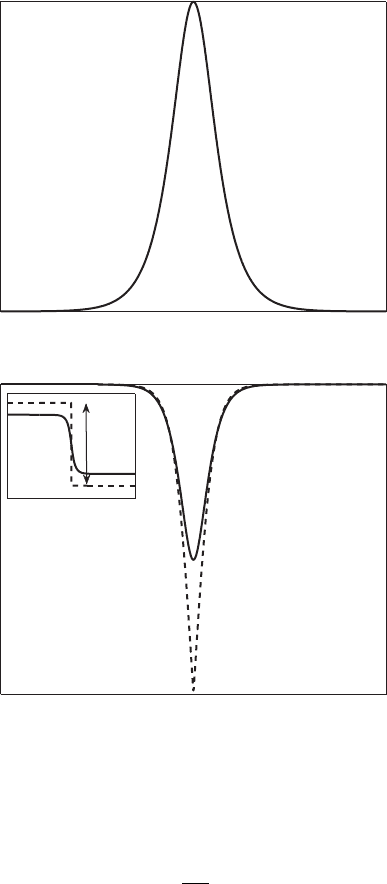
arbitrary real parameters. In Figure 6.1 a “bright” and the two
dark (black and gray) are depicted.
These solutions satisfy the boundary conditions
u(x, t) → u
±
(t) = ηe
2iη
2
t+iψ
0
±iα
as x →±∞
and appear as localized dips of intensity η
2
sin
2
α on the background field η.
The gray soliton moves with velocity 2η cos α and reduces to the dark (black)
soliton when α → π/2 with ψ
0
= −π/2(Hasegawa and Tappert, 1973b;
Zakharov and Shabat, 1973); see also Prinari et al. (2006) where the vector
IST problem for non-decaying data is discussed in detail.
A property of the NLS equation we will investigate next is its Galilean
invariance. That is, if u
1
(x, t) is a solution of (6.47) then so is
u
2
(x, t) = u
1
(x − vt, t)e
i
(
kx−ωt
)
,
with k = v/2 and ω = k
2
. Substituting u
2
into (6.47) we find u
1
satisfies:
iu
1,t
+ ωu
1
− ivu
1,x
+ (u
1,xx
+ 2iku
1,x
− k
2
u
1
) + 2|u
1
|
2
u
1
= 0.
Using the fact that u
1
is assumed to be a solution of (6.47) and using the values
for k,ω, this implies u
2
also satisfies (6.47).
154 Nonlinear Schr¨odinger models and water waves
π
black soliton
gray soliton
Figure 6.1 Bright (top) and dark (bottom) solitons of the NLS. In the inset
we plot the relative phases.
Another important result involves the linear stability of a special periodic
solution of (6.47). In (6.45a), i.e., the standard water wave formulation, take A
independent of ξ to get
iA
τ
=
2k
4
ω
|A|
2
A.
Note that this agrees with the results of the Stoke’s frequency shift calculation,
(6.33). With the change of variables mentioned above in terms of the standard
NLS, (6.47), this means:
iu
t
= −2|u|
2
u,