Wooldridge J., Introductory Econometrics - A Modern Approach (Instructors Manual)

Подождите немного. Документ загружается.

= –.040 – .222 log(price



gprice

t-1

) + .00097 t

(.019) (.092) (.00049)

+ .328 gprice

t-1

+ .130 gprice

t-2

(.155) (.149)

n = 39, R

= .200,

Now the Dickey-Fuller t statistic is about –2.41, which is above –3.12, the 10% critical value

from Table 18.3. [The estimated root is 1 – .222 = .778, which is much larger than for

log(invpc

).] We cannot reject the unit root null at a sufficiently small significance level.

(iii) Given the very strong evidence that log(invpc

) does not contain a unit root, while

log(price

) may very well, it makes no sense to discuss cointegration between the two. If we take

any nontrivial linear combination of an I(0) process (which may have a trend) and an I(1) process,

the result will be an I(1) process (possibly with drift).

18.12 (i) The estimated AR(3) model for pcip



cip

= 1.80 + .349 pcip

t-1

+ .071 pcip

t-2

+ .067 pcip

t-2

(0.55) (.043) (.045) (.043)

n = 554, R

= .166,

= 12.15.

When pcip

t-4

is added, its coefficient is .0043 with a t statistic of about .10.

(ii) In the model

pcip

t-1

pcip

t-2

pcip

t-3

pcsp

t-1

pcsp

t-2

pcsp

t-3

+ u

The null hypothesis is that pcsp does not Granger cause pcip. This is stated as H

0. The F statistic for joint significance of the three lags of pcsp

, with 3 and 547 df, is F = 5.37

and p-value = .0012. Therefore, we strongly reject H

and conclude that pcsp does Granger

cause pcip.

(iii) When we add Δi3

t-1

, Δi3

t-2

, and Δi3

t-3

to the regression from part (ii), and now test the

joint significance of pcsp

t-1

, pcsp

t-2

, and pcsp

t-3

, the F statistic is 5.08. With 3 and 544 df in the F

distribution, this gives p-value = .0018, and so pcsp Granger causes pcip even conditional on

past Δi3.

[Instructor’s Note: The F test for joint significance of Δi3

t-1

, Δi3

t-2

, and Δi3

t-3

yields p-

value = .228, and so Δi3 does not Granger cause pcip conditional on past pcsp.]

18.13 We first run the regression gfr

on pe

, t, and t

, and obtain the residuals, . We then

apply the augmented Dickey-Fuller test, with one lag of Δ , by regressing Δ on and

−

183

Δ . There are 70 observations available for this last regression, and it yields −.165 as the

coefficient on with t statistic = −2.76. This is well above –4.15, the 5% critical value

[obtained from Davidson and MacKinnon (1993, Table 20.2)]. Therefore, we cannot reject the

null hypothesis of no cointegration, so we conclude gfr

−

and pe

are not cointegrated even if we

allow them to have different quadratic trends.

18.14 (i) The estimated equation is

= .078 + 1.027 hy3

t-1

− 1.021 Δhy3

− .085 Δhy3

t-1

− .104 Δhy3

t-2

(.028) (0.016) (0.038) (.037) (.037)

n = 121, R

= .982,

= .123.

The t statistic for H

= 1 is (1.027 – 1)/.016

≈

1.69. We do not reject H

= 1 at the 5% level

against a two-sided alternative, although we would reject at the 10% level.

[Instructor’s Note: The standard errors on all slope coefficients can be used to construct t

statistics with approximate t distributions, provided there is no serial correlation in {e

}.]

(ii) The estimated error correction model is

= .070 + 1.259 Δhy3

t-1

− .816 (hy6

t-1

– hy3

t-2

)

(.049) (.278) (.256)

+ .283 Δhy3

t-2

+ .127 (hy6

t-2

– hy3

t-3

)

(.272) (.256)

n = 121, R

= .795.

Neither of the added terms is individually significant. The F test for their joint significance gives

F = 1.35, p-value = .264. Therefore, we would omit these terms and stick with the error

correction model estimated in (18.39).

18.15 (i) The updated equations using data through 1997 are

= 1.549 + .734 unem



unem

t-1

(0.572) (.096)

n = 49, R

= .554,

= 1.041

and

= 1.286 + .648 unem



unem

t-1

+ .185 inf

t-1

(0.484) (.083) (.041)

n = 49, R

= .691,

= .876.

184

The parameter estimates do not change by much. This is not very surprising, as we have added

only one year of data.

(ii) The forecast for unem

1998

from the first equation is 1.549 + .734(4.9)

5.15; from the

second equation the forecast is 1.286 + .648(4.9) + .185(2.3)

≈

4.89. The actual civilian

unemployment rate for 1998 was 4.5 (from Table B-42 in the 1999 Economic Report of the

President). Once again the model that includes lagged inflation produces a better forecast.

(iii) There is no practical improvement in reestimating the parameters using data through

1997: 4.89 versus 4.90, which differs in a digit that is not even reported in the published

unemployment series.

(iv) To obtain the two-step-ahead forecast we need the 1996 unemployment rate, which was

5.4. From equation (18.55), the forecast of unem

1998

made after we know unem

1996

(1 + .732)(1.572) + (.732

)(5.4)

5.62. The one-step ahead forecast is 1.572 + .732(4.9)

≈

5.16,

and so it is better to use the one-step-ahead forecast, as it is much closer to 4.5.

18.16 (i) The estimated linear trend equation using the first 119 observations is

= 248.58 + 5.15 t



chnimp

(53.20) (0.77)

n = 119, R

= .277,

= 288.33.

The standard error of the regression is 288.33.

(ii) The estimated AR(1) model excluding the last 12 months is

= 329.18 + .416 chnimp



chnimp

t-1

(54.71) (.084)

n = 118, R

= .174,

= 308.17.

Because

is lower for the linear trend model, it provides the better in-sample fit. (The R-

squared is also larger for the linear trend model.)

(iii) Using the last 12 observations for one-step-ahead out-of-sample forecasting gives an

RMSE and MAE for the linear trend equation of about 315.5 and 201.9, respectively. For the

AR(1) model, the RMSE and MAE are about 388.6 and 246.1, respectively. Perhaps

surprisingly, the linear trend is the better forecasting model.

(iv) Using again the first 119 observations, the F statistic for joint significance of feb

mar

, …, dec

when added to the linear trend model is about 1.15 with p-value

≈

.328. (The df

are 11 and 107.) So there is no evidence that seasonality needs to be accounted for in forecasting

chnimp.

185

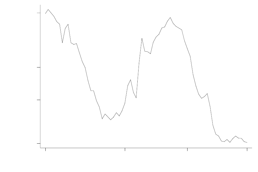
18.17 (i) As can be seen from the following graph, gfr does not have a clear upward or

downward trend. Starting from 1913, there is a sharp downward trend in fertility until the mid-

1930s, when the fertility rate bottoms out. Fertility increased markedly until the end of the baby

boom in the early 1960s, after which point it fell sharply and then leveled off.

year

1913

1941 1963 1984

100

gfr

125

(ii) The regression of gfr

on a cubic in t, using the data up through 1979, gives

= 148.71 - 6.90 t + .243 t

gfr

− .0024 t

(5.09) (0.64) (.022) (.0002)

n = 67, R

= .739,

= 9.84.

If we use the usual t critical values, all terms are very statistically significant, and the R-squared

indicates that this curve-fitting exercise tracks gfr

pretty well, at least up through 1979.

(iii) The MAE is about 43.02.

(iv) The regression Δgfr

on just an intercept, using data up through 1979, gives

= –.871

gfrΔ

(.543)

n = 66,

= 4.41.

186

(The R-squared is identically zero since there are no explanatory variables. But

, which

estimates the standard deviation of the error, is comparable to that in part (ii), and we see that it

is much smaller here.) The t statistic for the intercept is about –1.60, which is not significant at

the 10% level against a two-sided alternative. Therefore, it is legitimate to treat gfr

as having no

drift, if it is indeed a random walk. (That is, if gfr

+ gfr

t-1

+ e

, where {e

} is zero-mean,

serially uncorrelated process, then we cannot reject H

= 0.)

(v) The prediction of gfr

n+1

is simply gfr

, so the predication error is simply Δgfr

n+1

= gfr

n+1

–

gfr

. Obtaining the MAE for the five prediction errors for 1980 through 1984 gives MAE

≈

.840,

which is much lower than the 43.02 obtained with the cubic trend model. The random walk is

clearly preferred for forecasting.

(vi) The estimated AR(2) model for gfr

= 3.22 + 1.272 gfr

gfr

t-1

– .311 gfr

t-2

(2.92) (0.120) (.121)

n = 65, R

= .949,

= 4.25.

The second lag is significant. (Recall that its t statistic is valid even though gfr

apparently

contains a unit root: the coefficients on the two lags sum to .961.) The standard error of the

regression is slightly below that of the random walk model.

(vii) The out-of-sample forecasting performance of the AR(2) model is worse than the

random walk without drift: the MAE for 1980 through 1984 is about .991 for the AR(2) model.

[Instructor’s Note: You might have the students compare an AR(1) model for ∆gfr

− that is,

impose the unit root − to the random walk without drift model. The MAE is about .879, so it is

better to impose the unit root. But this still does less well than the simple random walk without

drift.]

18.18 (i) Using the data up through 1989 gives

= 3,186.04 + 116.24 t + .630 y

t-1

(1,163.09) (46.31) (.148)

n = 30, R

= .994,

= 223.95.

(Notice how high the R-squared is. However, it is meaningless as a goodness-of-fit measure

because {y

} has a trend and possibly a unit root.)

(ii) The forecast for 1990 (t = 32) is 3,186.04 + 116.24(32) + .630(17,804.09)

18,122.30,

because y is $17,804.09 in 1989. The actual value for real per capita disposable income was

$17,944.64, and so the forecast error is –$177.66.

≈

(iii) The MAE for the 1990s, using the model estimated in part (i), is about 371.76.

187

(iv) Without y

t-1

in the equation, we obtain

= 8,143.11 + 311.26 t

(103.38) (5.64)

n = 31, R

= .991,

= 280.87.

The MAE for the forecasts in the 1990s is about 718.26. This is much higher than for the model

with y

t-1

, so we should use the AR(1) model with a linear time trend.

18.19 (i) The AR(1) model for Δr6, estimated using all but the last 16 observations, is

= .047 – .179 Δr6



r6Δ

t-1

(.131) (.096)

n = 106, R

= .032,

= .023.

The RMSE for forecasting one-step-ahead over the last 16 quarters is about .704.

(ii) The equation with spr

t-1

included is

= .372 – .171 Δr6



r6Δ

t-1

– 1.045 spr

t-1

(.195) (.095) (0.474)

n = 106, R

= .076,

R = .058.

The RMSE is about .788, which is higher than the RMSE without the error correction term.

Therefore, while the EC term improves the in-sample fit (and is statistically significant), it

actually hampers out-of-sample forecasting.

(iii) To make the forecasting exercises comparable, we exclude the last 16 observations to

estimate the cointegrating parameters. The CI coefficient is about 1.028. The estimated error

correction model is

= .372 – .171 Δr6



r6Δ

t-1

– 1.045 (r6

t-1

– 1.028 r3

t-1

)

(.195) (.095) (0.474)

n = 106, R

= .058,

= .040,

which shows that this fits worse than the EC model when the cointegrating parameter is assumed

to be one. The RMSE for the last 16 quarters is .782, so this works slightly better. But both

versions of the EC model are dominated by the AR(1) model for Δr6

[Instructor’s Note: Since Δr6

t-1

is only marginally significant in the AR(1) model, and its

coefficient is small, and the intercept is also very small and insignificant, you might have the

188

students use zero to predict Δr6 for each of the last 16 quarters. The RMSE is about .657, which

means this works best of all. The lesson is that econometric methods are not always called for,

or even desirable.]

(iv) The conclusions would be identical because, as shown in Problem 18.9, the one-step-

ahead errors for forecasting r6

n+1

are identical to those for forecasting Δr6

n+1

18.20 (i) For lsp500, the ADF statistic without a trend is t = −.79; with a trend, the t statistic is

−2.20. This are both well above their respective 10% critical values. In addition, the estimated

roots are quite close to one. For lip, the ADF statistic without a trend is −1.37 without a trend

and −2.52 with a trend. Again, these are not close to rejecting even at the 10% levels, and the

estimated roots are very close to one.

(ii) The simple regression of lsp500 on lip gives

−2.402 + 1.694 lip



500lsp =

(.095) (.024)

n = 558, R

= .903

The t statistic for lip is over 70, and the R-squared is over .9. These are hallmarks of spurious

regressions.

(iii) Using the residuals obtained in part (ii), the ADF statistic (with two lagged changes)

is −1.57, and the estimated root is over .99. There is no evidence of cointegration. (The 10%

critical value is −3.04.)

(iv) After adding a linear time trend to the regression from part (ii), the ADF statistic applied

to the residuals is −1.88, and the estimated root is again about .99. Even with a time trend there

is no evidence of cointegration.

(v) It appears that lsp500 and lip do not move together in the sense of cointegration, even if

we allow them to have unrestricted linear time trends. This analysis does not point to a long-run

equilibrium relationship.

18.21 (i) This is supposed to be an AR(3) model, otherwise the claim is incorrect. So, estimating

an AR(3) for pcip

, and computing the F statistic for the second and third lags, gives F(2,550) =

3.76, p-value = .024.

(ii) When pcsp

t-1

is added to the AR(3) model in part (i), its coefficient is about .031 and its

t statistic is about 2.40. Therefore, we conclude that pcsp does Granger cause pcip.

(iii) The heteroskedasticity-robust t statistic is 2.47, so the conclusion from part (ii) does not

change.

189

18.22 (i) The DF statistic is about −3.31, which is above the 2.5% critical value (−3.12), and so,

using this test, we can reject a unit root at the 2.5% level. (The estimated root is about .81.)

(ii) When two lagged changes are added to the regression in part (i), the t statistic becomes

−1.50, and the root is larger (about .915). Now, there is little evidence against a unit root.

(iii) If we add a time trend to the regression in part (ii), the ADF statistic becomes −3.67, and

the estimated root is about .57. The 2.5% critical value is −3.66, and so we are back to fairly

convincingly rejecting a unit root.

(iv) The best characterization seems to be an I(0) process about a linear trend. In fact, a

stable AR(3) about a linear trend is suggested by the regression in part (iii).

(v) For prcfat

, the ADF statistic without a trend is −4.74 (estimated root = .62) and with a

time trend the statistic is −5.29 (estimated root = .54). Here, the evidence is strongly in favor of

an I(0) process, whether we include a trend or not.

190

CHAPTER 19

TEACHING NOTES

This is a chapter that students should read if you have assigned them a term paper. I used to

allow students to choose their own topics, but this is difficult in a first-semester course, and

places a heavy burden on instructors or teaching assistants, or both. I now assign a common

topic and provide a data set with about six weeks left in the term. The data set is cross-sectional

(because I teach time series at the end of the course), and I provide guidelines of the kinds of

questions students should try to answer. (For example, I might ask them to answer the following

questions: Is there a marriage premium for NBA basketball players? If so, does it depend on

race? Can the premium, if it exists, be explained by productivity differences?) The specifics are

up to the students, and they are to craft a 10 to 15-page paper on their own. This gives them

practice writing up the results in a way that is easy-to-read, and forces them to interpret their

findings. While leaving the topic to each student’s discretion is more interesting, I find that

many students flounder with an open-ended assignment until it is too late. Naturally, for a

second-semester course, or a senior seminar, students would be expected to design their own

topic, collect their own data, and then write a more substantial term paper.

191

APPENDIX A

SOLUTIONS TO PROBLEMS

A.1 (i) $566.

(ii) The two middle numbers are 480 and 530; when these are averaged, we obtain 505, or

$505.

(iii) 5.66 and 5.05, respectively.

(iv) The average increases to $586 while the median is unchanged ($505).

A.2 (i) This is just a standard linear equation with intercept equal to 3 and slope equal to .2. The

intercept is the number of missed classes for a student who lives on campus.

(ii) 3 + .2(5) = 4 classes.

(iii) 10(.2) = 2 classes.

A.3 If price = 15 and income = 200, quantity = 120 – 9.8(15) + .03(200) = –21, which is

nonsense. This shows that linear demand functions generally cannot describe demand over a

wide range of prices and income.

A.4 (i) The percentage point change is 5.6 – 6.4 = –.8, or an eight-tenths of a percentage point

decrease in the unemployment rate.

(ii) The percentage change in the unemployment rate is 100[(5.6 – 6.4)/6.4] = –12.5%.

A.5 The majority shareholder is referring to the percentage point increase in the stock return,

while the CEO is referring to the change relative to the initial return of 15%. To be precise, the

shareholder should specifically refer to a 3 percentage point increase.

A.6 (i) 100[42,000 – 35,000)/35,000] = 20%.

(ii) The approximate proportionate change is log(42,000) – log(35,000) .182, so the

approximate percentage change is %18.2. [Note: log(⋅) denotes the natural log.]

≈

A.7 (i) When exper = 0, log(salary) = 10.6; therefore, salary = exp(10.6)

≈

$40,134.84. When

exper = 5, salary = exp[10.6 + .027(5)]

≈

$45,935.80.

(ii) The approximate proportionate increase is .027(5) = .135, so the approximate percentage

change is 13.5%.

(iii) 100[(45,935.80 – 40,134.84)/40,134.84)

≈

14.5%, so the exact percentage increase is

about one percentage point higher.

192