Wooldridge J. Introductory Econometrics: A Modern Approach (Basic Text - 3d ed.)
Подождите немного. Документ загружается.

this is to use the n observations to regress y
t
on exp(logy
t
)without an intercept. Let
ˆ
be
the slope coefficient on exp(logy
t
). Then, the forecast of y in period n h is simply
f
ˆ
n,h
ˆ
exp[
ˆ
ˆ
(n h)]. (18.62)
As an example, if we use the first 687 weeks of data on the New York Stock Exchange
index in NYSE.RAW, we obtain
ˆ
3.782 and
ˆ
.0019 [by regressing log(price
t
) on
a linear time trend]; this shows that the index grows about .2% per week, on average. When
we regress price on the exponentiated fitted values, we obtain
ˆ
1.018. Now, we fore-
cast price four weeks out, which is the last week in the sample, using (18.62):
1.018exp[3.782 .0019(691)] 166.12. The actual value turned out to be 164.25, so
we have somewhat overpredicted. But this result is much better than if we estimate a lin-
ear time trend for the first 687 weeks: the forecasted value for week 691 is 152.23, which
is a substantial underprediction.
Although trend models can be useful for prediction, they must be used with caution,
especially for forecasting far into the future integrated series that have drift. The poten-
tial problem can be seen by considering a random walk with drift. At time t h,we
can write y
th
as
y
th
h y
t
u
t1
… u
th
,
666 Part 3 Advanced Topics
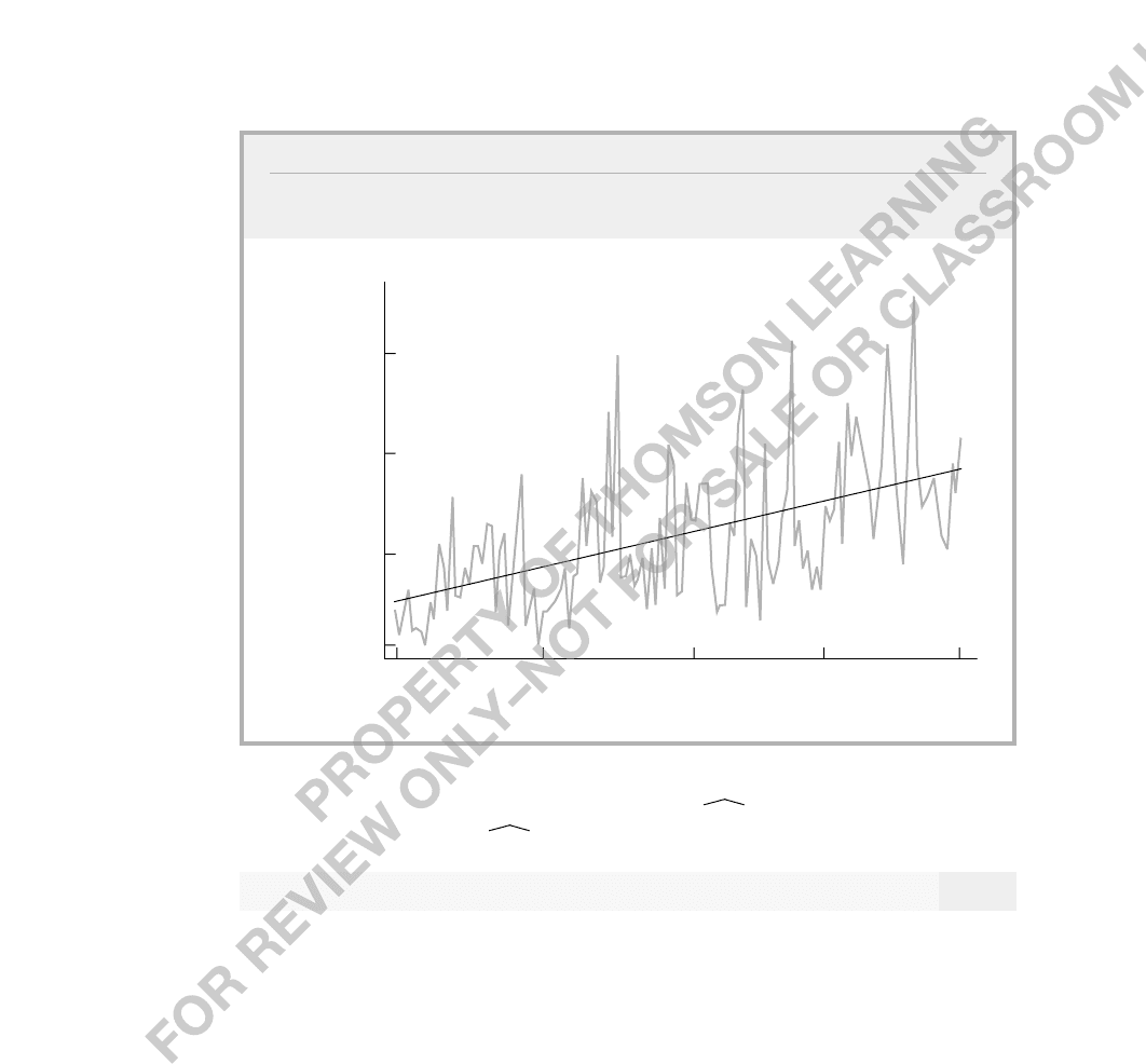
FIGURE 18.2
Chinese barium chloride imports into the United States (in short tons) and its
estimated linear trend line, 249.56 5.15t.
barium
chloride
(short tons)
131
100
t
7035
1
40
500
1000
1500

Chapter 18 Advanced Time Series Topics 667
where
is the drift term (usually
0), and each u
tj
has zero mean given I
t
and con-
stant variance
2
. As we saw earlier, the forecast of y
th
at time t is E(y
th
I
t
)
h y
t
,
and the forecast error variance is
2
h. What happens if we use a linear trend model? Let
y
0
be the initial value of the process at time zero, which we take as nonrandom. Then, we
can also write
y
th
y
0
(t h) u
1
u
2
… u
th
y
0
(t h) v
th
.
This looks like a linear trend model with the intercept
y
0
. But the error, v
th
,while
having mean zero, has variance
2
(t h). Therefore, if we use the linear trend
y
0
(t h) to forecast y
th
at time t, the forecast error variance is
2
(t h), compared
with
2
h when we use
h y
t
. The ratio of the forecast variances is (t h)/h,which can
be big for large t. The bottom line is that we should not use a linear trend to forecast a
random walk with drift. (Computer Exercise C18.8 asks you to compare forecasts from a
cubic trend line and those from the simple random walk model for the general fertility rate
in the United States.)
Deterministic trends can also produce poor forecasts if the trend parameters are esti-
mated using old data and the process has a subsequent shift in the trend line. Sometimes,
exogenous shocks—such as the oil crises of the 1970s—can change the trajectory of trend-
ing variables. If an old trend line is used to forecast far into the future, the forecasts can
be way off. This problem can be mitigated by using the most recent data available to obtain
the trend line parameters.
Nothing prevents us from combining trends with other models for forecasting. For
example, we can add a linear trend to an AR(1) model, which can work well for forecast-
ing series with linear trends but which are also stable AR processes around the trend.
It is also straightforward to forecast processes with deterministic seasonality (monthly
or quarterly series). For example, the file BARIUM.RAW contains the monthly production
of gasoline in the United States from 1978 through 1988. This series has no obvious trend,
but it does have a strong seasonal pattern. (Gasoline production is higher in the summer
months and in December.) In the simplest model, we would regress gas (measured in gal-
lons) on 11 month dummies, say, for February through December. Then, the forecast for
any future month is simply the intercept plus the coefficient on the appropriate month
dummy. (For January, the forecast is just the intercept in the regression.) We can also add
lags of variables and time trends to allow for general series with seasonality.
Forecasting processes with unit roots also deserves special attention. Earlier, we
obtained the expected value of a random walk conditional on information through time n.
To forecast a random walk, with possible drift
, h periods into the future at time n,we
use f
ˆ
n,h
ˆ
h y
n
,where
ˆ
is the sample average of the y
t
up through t n. (If there
is no drift, we set
ˆ
0.) This approach imposes the unit root. An alternative would be
to estimate an AR(1) model for {y
t
} and to use the forecast formula (18.55). This approach
does not impose a unit root, but if one is present,
ˆ
converges in probability to one as n
gets large. Nevertheless,
ˆ
can be substantially different than one, especially if the sam-
ple size is not very large. The matter of which approach produces better out-of-sample
forecasts is an empirical issue. If in the AR(1) model,
is less than one, even slightly, the
AR(1) model will tend to produce better long-run forecasts.

Generally, there are two approaches to producing forecasts for I(1) processes. The first
is to impose a unit root. For a one-step-ahead forecast, we obtain a model to forecast the
change in y, y
t1
,given information through time t. Then, because y
t1
y
t1
y
t
,
E(y
t1
I
t
) E(y
t1
I
t
) y
t
. Therefore, our forecast of y
n1
at time n is just
f
ˆ
n
g
ˆ
n
y
n
,
where g
ˆ
n
is the forecast of y
n1
at time n. Typically, an AR model (which is necessarily
stable) is used for y
t
, or a vector autoregression.
This can be extended to multiple-step-ahead forecasts by writing y
nh
as
y
nh
(y
nh
y
nh1
) (y
nh1
y
nh2
) … (y
n1
y
n
) y
n
,
or
y
nh
y
nh
y
nh1
… y
n1
y
n
.
Therefore, the forecast of y
nh
at time n is
f
ˆ
n,h
g
ˆ
n,h
g
ˆ
n,h1
… g
ˆ
n,1
y
n
, (18.63)
where g
ˆ
n,j
is the forecast of y
nj
at time n. For example, we might model y
t
as a stable
AR(1), obtain the multiple-step-ahead forecasts from (18.55) (but with
ˆ
and
ˆ
obtained
from y
t
on y
t1
, and y
n
replaced with y
n
), and then plug these into (18.63).
The second approach to forecasting I(1) variables is to use a general AR or VAR model
for {y
t
}. This does not impose the unit root. For example, if we use an AR(2) model,
y
t
1
y
t1
2
y
t2
u
t
, (18.64)
then
1
2
1. If we plug in
1
1
2
and rearrange, we obtain y
t
2
y
t1
u
t
,which is a stable AR(1) model in the difference that takes us back to the first
approach described earlier. Nothing prevents us from estimating (18.64) directly by OLS.
One nice thing about this regression is that we can use the usual t statistic on
ˆ
2
to deter-
mine if y
t2
is significant. (This assumes that the homoskedasticity assumption holds; if
not, we can use the heteroskedasticity-robust form.) We will not show this formally, but,
intuitively, it follows by rewriting the equation as y
t
y
t1
2
y
t1
u
t
,where
1
2
. Even if
1,
2
is minus the coefficient on a stationary, weakly dependent
process {y
t1
}. Because the regression results will be identical to (18.64), we can use
(18.64) directly.
As an example, let us estimate an AR(2) model for the general fertility rate in
FERTIL3.RAW, using the observations through 1979. (In Computer Exercise C18.8, you
are asked to use this model for forecasting, which is why we save some observations at
the end of the sample.)
gfr
t
(3.22((1.272(gfr
t1
(.311(gfr
t2
gf
ˆ
r
t
(2.92)1(.120)gfr
t1
(.121)gfr
t2
n 65, R
2
.949, R
¯
2
.947.
(18.65)
668 Part 3 Advanced Topics

Chapter 18 Advanced Time Series Topics 669
The t statistic on the second lag is about 2.57, which is statistically different from zero
at about the 1% level. (The first lag also has a very significant t statistic, which has an
approximate t distribution by the same reasoning used for
ˆ
2
.) The R-squared, adjusted or
not, is not especially informative as a goodness-of-fit measure because gfr apparently con-
tains a unit root, and it makes little sense to ask how much of the variance in gfr we are
explaining.
The coefficients on the two lags in (18.65) add up to .961, which is close to and not
statistically different from one (as can be verified by applying the augmented Dickey-Fuller
test to the equation gfr
t
gfr
t1
1
gfr
t1
u
t
). Even though we have
not imposed the unit root restriction, we can still use (18.65) for forecasting, as we
discussed earlier.
Before ending this section, we point out one potential improvement in forecasting in
the context of vector autoregressive models with I(1) variables. Suppose {y
t
} and {z
t
} are
each I(1) processes. One approach for obtaining forecasts of y is to estimate a bivariate
autoregression in the variables y
t
and z
t
and then to use (18.63) to generate one- or
multiple-step-ahead forecasts; this is essentially the first approach we described earlier.
However, if y
t
and z
t
are cointegrated, we have more stationary, stable variables in the
information set that can be used in forecasting y: namely, lags of y
t
z
t
,where
is
the cointegrating parameter. A simple error correction model is
y
t
0
1
y
t1
1
z
t1
1
(y
t1
z
t1
) e
t
,
E(e
t
I
t1
) 0.
(18.66)
To forecast y
n1
, we use observations up through n to estimate the cointegrating parame-
ter,
, and then estimate the parameters of the error correction model by OLS, as described
in Section 18.4. Forecasting y
n1
is easy: we just plug y
n
, z
n
, and y
n
ˆ
z
n
into the
estimated equation. Having obtained the forecast of y
n1
, we add it to y
n
.
By rearranging the error correction model, we can write
y
t
0
1
y
t1
2
y
t2
1
z
t1
2
z
t2
u
t
,
(18.67)
where
1
1
1
,
2
1
, and so on, which is the first equation in a VAR model
for y
t
and z
t
. Notice that this depends on five parameters, just as many as in the error cor-
rection model. The point is that, for the purposes of forecasting, the VAR model in the
levels and the error correction model are essentially the same. This is not the case in more
general error correction models. For example, suppose that
1
1
0 in (18.66), but
we have a second error correction term,
2
(y
t2
z
t2
). Then, the error correction model
involves only four parameters, whereas (18.67)—which has the same order of lags for y
and z—contains five parameters. Thus, error correction models can economize on param-
eters; that is, they are generally more parsimonious than VARs in levels.
If y
t
and z
t
are I(1) but not cointegrated, the appropriate model is (18.66) without the
error correction term. This can be used to forecast y
n1
, and we can add this to y
n
to
forecast y
n1
.

670 Part 3 Advanced Topics
SUMMARY
The time series topics covered in this chapter are used routinely in empirical macroeco-
nomics, empirical finance, and a variety of other applied fields. We began by showing how
infinite distributed lag models can be interpreted and estimated. These can provide flexi-
ble lag distributions with fewer parameters than a similar finite distributed lag model. The
geometric distributed lag and, more generally, rational distributed lag models are the most
popular. They can be estimated using standard econometric procedures on simple dynamic
equations.
Testing for a unit root has become very common in time series econometrics. If a series
has a unit root, then, in many cases, the usual large sample normal approximations are no
longer valid. In addition, a unit root process has the property that an innovation has a long-
lasting effect, which is of interest in its own right. While there are many tests for unit roots,
the Dickey-Fuller t test—and its extension, the augmented Dickey-Fuller test—is proba-
bly the most popular and easiest to implement. We can allow for a linear trend when test-
ing for unit roots by adding a trend to the Dickey-Fuller regression.
When an I(1) series, y
t
, is regressed on another I(1) series, x
t
, there is serious concern
about spurious regression, even if the series do not contain obvious trends. This has been
studied thoroughly in the case of a random walk: even if the two random walks are inde-
pendent, the usual t test for significance of the slope coefficient, based on the usual criti-
cal values, will reject much more than the nominal size of the test. In addition, the R
2
tends
to a random variable, rather than to zero (as would be the case if we regress the differ-
ence in y
t
on the difference in x
t
).
In one important case, a regression involving I(1) variables is not spurious, and that is
when the series are cointegrated. This means that a linear function of the two I(1) vari-
ables is I(0). If y
t
and x
t
are I(1) but y
t
x
t
is I(0), y
t
and x
t
cannot drift arbitrarily far
apart. There are simple tests of the null of no cointegration against the alternative of coin-
tegration, one of which is based on applying a Dickey-Fuller unit root test to the residu-
als from a static regression. There are also simple estimators of the cointegrating param-
eter that yield t statistics with approximate standard normal distributions (and
asymptotically valid confidence intervals). We covered the leads and lags estimator in Sec-
tion 18.4.
Cointegration between y
t
and x
t
implies that error correction terms may appear in a
model relating y
t
to x
t
; the error correction terms are lags in y
t
x
t
,where
is the
cointegrating parameter. A simple two-step estimation procedure is available for estimat-
ing error correction models. First,
is estimated using a static regression (or the leads and
lags regression). Then, OLS is used to estimate a simple dynamic model in first differ-
ences that includes the error correction terms.
Section 18.5 contained an introduction to forecasting, with emphasis on regression-
based forecasting methods. Static models or, more generally, models that contain explana-
tory variables dated contemporaneously with the dependent variable, are limited because
then the explanatory variables need to be forecasted. If we plug in hypothesized values of
unknown future explanatory variables, we obtain a conditional forecast. Unconditional
forecasts are similar to simply modeling y
t
as a function of past information we have
observed at the time the forecast is needed. Dynamic regression models, including autore-
gressions and vector autoregressions, are used routinely. In addition to obtaining one-step-

Chapter 18 Advanced Time Series Topics 671
PROBLEMS
18.1 Consider equation (18.15) with k 2. Using the IV approach to estimating the
h
and
, what would you use as instruments for y
t1
?
18.2 An interesting economic model that leads to an econometric model with a lagged
dependent variable relates y
t
to the expected value of x
t
,say,x
t
*
,where the expectation is
based on all observed information at time t 1:
y
t
0
1
x
t
*
u
t
. (18.68)
ahead point forecasts, we also discussed the construction of forecast intervals, which are
very similar to prediction intervals.
Various criteria are used for choosing among forecasting methods. The most common
performance measures are the root mean squared error and the mean absolute error. Both
estimate the size of the average forecast error. It is most informative to compute these mea-
sures using out-of-sample forecasts.
Multiple-step-ahead forecasts present new challenges and are subject to large forecast
error variances. Nevertheless, for models such as autoregressions and vector autoregres-
sions, multi-step-ahead forecasts can be computed, and approximate forecast intervals can
be obtained.
Forecasting trending and I(1) series requires special care. Processes with determinis-
tic trends can be forecasted by including time trends in regression models, possibly with
lags of variables. A potential drawback is that deterministic trends can provide poor fore-
casts for long-horizon forecasts: once it is estimated, a linear trend continues to increase
or decrease. The typical approach to forecasting an I(1) process is to forecast the differ-
ence in the process and to add the level of the variable to that forecasted difference. Alter-
natively, vector autoregressive models can be used in the levels of the series. If the series
are cointegrated, error correction models can be used instead.
KEY TERMS
Augmented Dickey-Fuller
Test
Cointegration
Conditional Forecast
Dickey-Fuller Distribution
Dickey-Fuller (DF) Test
Engle-Granger Two-Step
Procedure
Error Correction Model
Exponential Smoothing
Forecast Error
Forecast Interval
Geometric (or Koyck)
Distributed Lag
Granger Causality
Infinite Distributed Lag
(IDL) Model
Information Set
In-Sample Criteria
Leads and Lags Estimator
Loss Function
Martingale
Martingale Difference
Sequence
Mean Absolute Error
(MAE)
Multiple-Step-Ahead
Forecast
One-Step-Ahead Forecast
Out-of-Sample Criteria
Point Forecast
Rational Distributed Lag
(RDL) Model
Root Mean Squared Error
(RMSE)
Spurious Regression
Problem
Unconditional Forecast
Unit Roots
Vector Autoregressive
(VAR) Model

A natural assumption on {u
t
} is that E(u
t
I
t1
) 0, where I
t1
denotes all information on
y and x observed at time t 1; this means that E(y
t
I
t1
)
0
1
x
t
*
. To complete this
model, we need an assumption about how the expectation x
t
*
is formed. We saw a simple
example of adaptive expectations in Section 11.2, where x
t
*
x
t1
. A more complicated
adaptive expectations scheme is
x
t
*
x
t
*
1
(x
t1
x
t
*
1
),
(18.69)
where 0
1. This equation implies that the change in expectations reacts to whether
last period’s realized value was above or below its expectation. The assumption 0
1
implies that the change in expectations is a fraction of last period’s error.
(i) Show that the two equations imply that
y
t
0
(1
)y
t1
1
x
t1
u
t
(1
)u
t1
.
[Hint: Lag equation (18.68) one period, multiply it by (1
), and sub-
tract this from (18.68). Then, use (18.69).]
(ii) Under E(u
t
I
t1
) 0, {u
t
} is serially uncorrelated. What does this imply
about the new errors, v
t
u
t
(1
)u
t1
?
(iii) If we write the equation from part (i) as
y
t
0
1
y
t1
2
x
t1
v
t
,
how would you consistently estimate the
j
?
(iv) Given consistent estimators of the
j
,how would you consistently esti-
mate
and
1
?
18.3 Suppose that {y
t
} and {z
t
} are I(1) series, but y
t
z
t
is I(0) for some
0. Show
that for any
, y
t
z
t
must be I(1).
18.4 Consider the error correction model in equation (18.37). Show that if you add
another lag of the error correction term, y
t2
x
t2
, the equation suffers from perfect
collinearity. (Hint: Show that y
t2
x
t2
is a perfect linear function of y
t1
x
t1
,
x
t1
, and y
t1
.)
18.5 Suppose the process {(x
t
,y
t
): t 0,1,2,…} satisfies the equations
y
t
x
t
u
t
and
x
t
x
t1
v
t
,
where E(u
t
I
t1
) E(v
t
I
t1
) 0, I
t1
contains information on x and y dated at time
t 1 and earlier,
0, and
1 [so that x
t
, and therefore y
t
, is I(1)]. Show that these
two equations imply an error correction model of the form
y
t
1
x
t1
(y
t1
x
t1
) e
t
,
where
1
,
1, and e
t
u
t
v
t
. (Hint: First subtract y
t1
from both sides
of the first equation. Then, add and subtract
x
t1
from the right-hand side and
672 Part 3 Advanced Topics

Chapter 18 Advanced Time Series Topics 673
rearrange. Finally, use the second equation to get the error correction model that con-
tains x
t1
.)
18.6 Using the monthly data in VOLAT.RAW, the following model was estimated:
pcip (1.54)(.344)pcip
1
(.074)pcip
2
(.073)pcip
3
(.031)pcsp
1
pci
ˆ
p 0(.56)(.042)pcip
1
(.045)pcip
2
(.042)pcip
3
(.013)pcsp
1
n 554, R
2
.174, R
¯
2
.168,
where pcip is the percentage change in monthly industrial production, at an annualized
rate, and pcsp is the percentage change in the Standard & Poor’s 500 Index, also at an
annualized rate.
(i) If the past three months of pcip are zero and pcsp
1
0, what is the pre-
dicted growth in industrial production for this month? Is it statistically
different from zero?
(ii) If the past three months of pcip are zero but pcsp
1
10, what is the
predicted growth in industrial production?
(iii) What do you conclude about the effects of the stock market on real eco-
nomic activity?
18.7 Let gM
t
be the annual growth in the money supply and let unem
t
be the unem-
ployment rate. Assuming that unem
t
follows a stable AR(1) process, explain in detail how
you would test whether gM Granger causes unem.
18.8 Suppose that y
t
follows the model
y
t
1
z
t1
u
t
u
t
u
t1
e
t
E(e
t
I
t1
) 0,
where I
t1
contains y and z dated at t 1 and earlier.
(i) Show that E(y
t1
I
t
) (1
)
y
t
1
z
t
1
z
t1
. (Hint:Write
u
t1
y
t1
1
z
t2
and plug this into the second equation; then,
plug the result into the first equation and take the conditional expecta-
tion.)
(ii) Suppose that you use n observations to estimate
,
1
, and
. Write the
equation for forecasting y
n1
.
(iii) Explain why the model with one lag of z and AR(1) serial correlation is
a special case of the model
y
t
0
y
t1
1
z
t1
2
z
t2
e
t
.
(iv) What does part (iii) suggest about using models with AR(1) serial cor-
relation for forecasting?
18.9 Let {y
t
} be an I(1) sequence. Suppose that g
ˆ
n
is the one-step-ahead forecast of
y
n1
and let f
ˆ
n
g
ˆ
n
y
n
be the one-step-ahead forecast of y
n1
. Explain why the fore-
cast errors for forecasting y
n1
and y
n1
are identical.

COMPUTER EXERCISES
C18.1 Use the data in WAGEPRC.RAW for this exercise. Problem 11.5 gave estimates
of a finite distributed lag model of gprice on gwage,where 12 lags of gwage are used.
(i) Estimate a simple geometric DL model of gprice on gwage. In partic-
ular, estimate equation (18.11) by OLS. What are the estimated impact
propensity and LRP? Sketch the estimated lag distribution.
(ii) Compare the estimated IP and LRP to those obtained in Problem 11.5.
How do the estimated lag distributions compare?
(iii) Now, estimate the rational distributed lag model from (18.16). Sketch
the lag distribution and compare the estimated IP and LRP to those
obtained in part (ii).
C18.2 Use the data in HSEINV.RAW for this exercise.
(i) Test for a unit root in log(invpc), including a linear time trend and two
lags of log(invpc
t
). Use a 5% significance level.
(ii) Use the approach from part (i) to test for a unit root in log(price).
(iii) Given the outcomes in parts (i) and (ii), does it make sense to test for
cointegration between log(invpc) and log(price)?
C18.3 Use the data in VOLAT.RAW for this exercise.
(i) Estimate an AR(3) model for pcip. Now, add a fourth lag and verify
that it is very insignificant.
(ii) To the AR(3) model from part (i), add three lags of pcsp to test whether
pcsp Granger causes pcip. Carefully, state your conclusion.
(iii) To the model in part (ii), add three lags of the change in i3, the three-
month T-bill rate. Does pcsp Granger cause pcip conditional on
past i3?
C18.4 In testing for cointegration between gfr and pe in Example 18.5, add t
2
to equa-
tion (18.32) to obtain the OLS residuals. Include one lag in the augmented DF test. The
5% critical value for the test is 4.15.
C18.5 Use INTQRT.RAW for this exercise.
(i) In Example 18.7, we estimated an error correction model for the hold-
ing yield on six-month T-bills, where one lag of the holding yield on
three-month T-bills is the explanatory variable. We assumed that the
cointegration parameter was one in the equation hy6
t
hy3
t1
u
t
. Now, add the lead change, hy3
t
, the contemporaneous change,
hy3
t1
, and the lagged change, hy3
t2
, of hy3
t1
. That is, estimate
the equation
hy6
t
hy3
t1
0
hy3
t
1
hy3
t1
1
hy3
t2
e
t
and report the results in equation form. Test H
0
:
1 against a two-
sided alternative. Assume that the lead and lag are sufficient so that
{hy3
t1
} is strictly exogenous in this equation and do not worry about
serial correlation.
674 Part 3 Advanced Topics

Chapter 18 Advanced Time Series Topics 675
(ii) To the error correction model in (18.39), add hy3
t2
and (hy6
t2
hy3
t3
). Are these terms jointly significant? What do you conclude
about the appropriate error correction model?
C18.6 Use the data in PHILLIPS.RAW to answer these questions.
(i) Estimate the models in (18.48) and (18.49) using the data through 1997.
Do the parameter estimates change much compared with (18.48) and
(18.49)?
(ii) Use the new equations to forecast unem
1998
; round to two places after
the decimal. Which equation produces a better forecast?
(iii) As we discussed in the text, the forecast for unem
1998
using (18.49) is
4.90. Compare this with the forecast obtained using the data through
1997. Does using the extra year of data to obtain the parameter esti-
mates produce a better forecast?
(iv) Use the model estimated in (18.48) to obtain a two-step-ahead forecast
of unem. That is, forecast unem
1998
using equation (18.55) with
ˆ
1.572,
ˆ
.732, and h 2. Is this better or worse than the one-
step-ahead forecast obtained by plugging unem
1997
4.9 into (18.48)?
C18.7 Use the data in BARIUM.RAW for this exercise.
(i) Estimate the linear trend model chnimp
t
t u
t
, using the first
119 observations (this excludes the last 12 months of observations for
1988). What is the standard error of the regression?
(ii) Now, estimate an AR(1) model for chnimp,again using all data but the
last 12 months. Compare the standard error of the regression with that
from part (i). Which model provides a better in-sample fit?
(iii) Use the models from parts (i) and (ii) to compute the one-step-ahead
forecast errors for the 12 months in 1988. (You should obtain 12 fore-
cast errors for each method.) Compute and compare the RMSEs and
the MAEs for the two methods. Which forecasting method works better
out-of-sample for one-step-ahead forecasts?
(iv) Add monthly dummy variables to the regression from part (i). Are these
jointly significant? (Do not worry about the slight serial correlation in
the errors from this regression when doing the joint test.)
C18.8 Use the data in FERTIL3.RAW for this exercise.
(i) Graph gfr against time. Does it contain a clear upward or downward
trend over the entire sample period?
(ii) Using the data through 1979, estimate a cubic time trend model for gfr
(that is, regress gfr on t, t
2
, and t
3
, along with an intercept). Comment
on the R-squared of the regression.
(iii) Using the model in part (ii), compute the mean absolute error of the
one-step-ahead forecast errors for the years 1980 through 1984.
(iv) Using the data through 1979, regress gfr
t
on a constant only. Is the con-
stant statistically different from zero? Does it make sense to assume that
any drift term is zero, if we assume that gfr
t
follows a random walk?