Wooldridge J. Introductory Econometrics: A Modern Approach (Basic Text - 3d ed.)
Подождите немного. Документ загружается.


which we can write as
y
t
0
z
t
y
t1
u
t
u
t1
, (18.10)
where
0
(1
)
. This equation looks like a standard model with a lagged dependent
variable, where z
t
appears contemporaneously. Because
is the coefficient on z
t
and
is the
coefficient on y
t1
,it appears that we can estimate these parameters. [If, for some reason,
we are interested in
, we can always obtain
ˆ
ˆ
0
/(1
ˆ
) after estimating
and
0
.]
The simplicity of (18.10) is somewhat misleading. The error term in this equation,
u
t
u
t1
, is generally correlated with y
t1
. From (18.9), it is pretty clear that u
t1
and
y
t1
are correlated. Therefore, if we write (18.10) as
y
t
0
z
t
y
t1
v
t
, (18.11)
where v
t
u
t
u
t1
, then we generally have correlation between v
t
and y
t1
. With-
out further assumptions, OLS estimation of (18.11) produces inconsistent estimates of
and
.
One case where v
t
must be correlated with y
t1
occurs when u
t
is independent of z
t
and
all past values of z and y. Then, (18.8) is dynamically complete, so u
t
is uncorrelated with
y
t1
. From (18.9), the covariance between v
t
and y
t1
is
Var(u
t1
)
u
2
,which is
zero only if
0. We can easily see that v
t
is serially correlated: because {u
t
} is serially
uncorrelated, E(v
t
v
t1
) E(u
t
u
t1
)
E(u
t
2
1
)
E(u
t
u
t2
)
2
E(u
t1
u
t2
)
u
2
. For
j 1, E(v
t
v
tj
) 0. Thus, {v
t
} is a moving average process of order one (see Section
11.1). This, and equation (18.11), gives an example of a model—which is derived from
the original model of interest—that has a lagged dependent variable and a particular kind
of serial correlation.
If we make the strict exogeneity assumption (18.5), then z
t
is uncorrelated with u
t
and
u
t1
, and therefore with v
t
. Thus, if we can find a suitable instrumental variable for y
t1
,
then we can estimate (18.11) by IV. What is a good IV candidate for y
t1
? By assump-
tion, u
t
and u
t1
are both uncorrelated with z
t1
, so v
t
is uncorrelated with z
t1
. If
0,
z
t1
and y
t1
are correlated, even after partialling out z
t
. Therefore, we can use instruments
(z
t
,z
t1
) to estimate (18.11). Generally, the standard errors need to be adjusted for serial
correlation in the {v
t
}, as we discussed in Section 15.7.
An alternative to IV estimation exploits the fact that {u
t
} may contain a specific kind
of serial correlation. In particular, in addition to (18.6), suppose that {u
t
} follows the
AR(1) model
u
t
u
t1
e
t
(18.12)
E(e
t
z
t
,y
t1
,z
t1
,…) 0. (18.13)
It is important to notice that the
appearing in (18.12) is the same parameter multiplying
y
t1
in (18.11). If (18.12) and (18.13) hold, we can write equation (18.10) as
y
t
0
z
t
y
t1
e
t
, (18.14)
636 Part 3 Advanced Topics

Chapter 18 Advanced Time Series Topics 637
which is a dynamically complete model under (18.13). From Chapter 11, we can obtain
consistent, asymptotically normal estimators of the parameters by OLS. This is very con-
venient, as there is no need to deal with serial correlation in the errors. If e
t
satisfies the
homoskedasticity assumption Var(e
t
z
t
,y
t1
)
e
2
, the usual inference applies. Once we
have estimated
and
, we can easily estimate the LRP: LRP
ˆ
/(1
ˆ
).
The simplicity of this procedure relies on the potentially strong assumption that {u
t
}
follows an AR(1) process with the same
appearing in (18.7). This is usually no worse
than assuming the {u
t
} are serially uncorrelated. Nevertheless, because consistency of the
estimators relies heavily on this assumption, it is a good idea to test it. A simple test begins
by specifying {u
t
} as an AR(1) process with a different parameter, say, u
t
u
t1
e
t
.
McClain and Wooldridge (1995) devised a simple Lagrange multiplier test of H
0
:
that can be computed after OLS estimation of (18.14).
The geometric distributed lag model extends to multiple explanatory variables—so that
we have an infinite DL in each explanatory variable—but then we must be able to write
the coefficient on z
tj,h
as
h
j
. In other words, though
h
is different for each explana-
tory variable,
is the same. Thus, we can write
y
t
0
1
z
t1
…
k
z
tk
y
t1
v
t
. (18.15)
The same issues that arose in the case with one z arise in the case with many z. Under the
natural extension of (18.12) and (18.13)—just replace z
t
with z
t
(z
t1
,…,z
tk
)—OLS is
consistent and asymptotically normal. Or, an IV method can be used.
Rational Distributed Lag Models
The geometric DL implies a fairly restrictive lag distribution. When
0 and
0, the
j
are positive and monotonically declining to zero. It is possible to have more general
infinite distributed lag models. The GDL is a special case of what is generally called a
rational distributed lag (RDL) model. A general treatment is beyond our scope—Har-
vey (1990) is a good reference—but we can cover one simple, useful extension.
Such an RDL model is most easily described by adding a lag of z to equation (18.11):
y
t
0
0
z
t
y
t1
1
z
t1
v
t
, (18.16)
where v
t
u
t
u
t1
, as before. By repeated substitution, it can be shown that (18.16)
is equivalent to the infinite distributed lag model
y
t
0
(z
t
z
t1
2
z
t2
…)
1
(z
t1
z
t2
2
z
t3
…) u
t
0
z
t
(
0
1
)z
t1
(
0
1
)z
t2
2
(
0
1
)z
t3
… u
t
,
where we again need the assumption
1. From this last equation, we can read off the
lag distribution. In particular, the impact propensity is
0
, while the coefficient on z
th
is
h1
(
0
1
) for h 1. Therefore, this model allows the impact propensity to differ in
638 Part 3 Advanced Topics
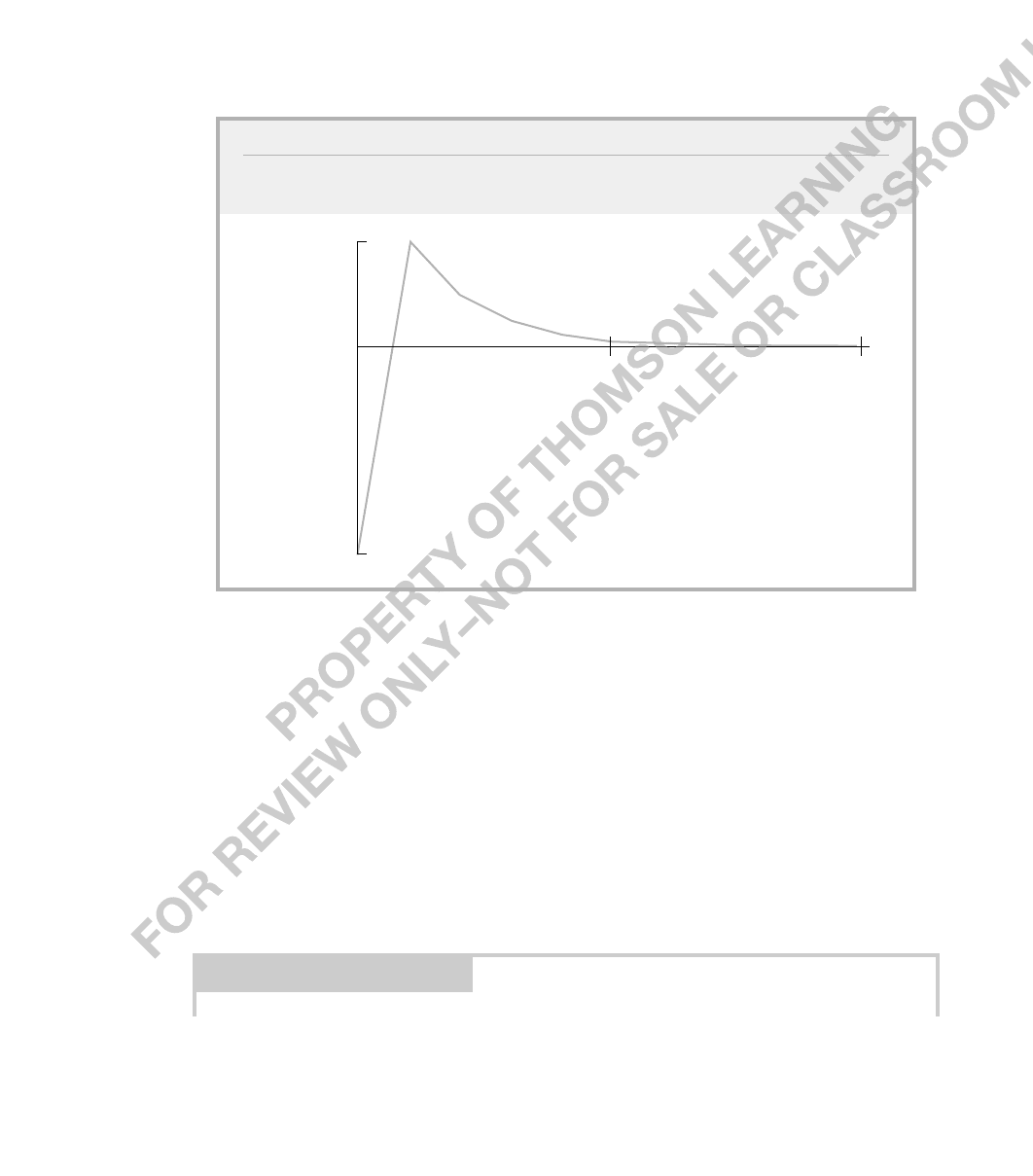
FIGURE 18.1
Lag distribution for the rational distributed lag (18.16) with
.5,
0
1,
and
1
1.
coefficient
.5
5
10
lag
1
0
sign from the other lag coefficients, even if
0. However, if
0, the
h
have the same
sign as (
0
1
) for all h 1. The lag distribution is plotted in Figure 18.1 for
.5,
0
1, and
1
1.
The easiest way to compute the long-run propensity is to set y and z at their long-run val-
ues for all t,say,y* and z*, and then find the change in y* with respect to z* (see also Prob-
lem 10.3). We have y*
0
0
z*
y*
1
z*, and solving gives y*
0
/(1
)
(
0
1
)/(1
)z*. Now, we use the fact that LRP y*/z*:
LRP (
0
1
)/(1
).
Because
1, the LRP has the same sign as
0
1
, and the LRP is zero if, and only
if,
0
1
0, as in Figure 18.1.
EXAMPLE 18.1
(Housing Investment and Residential Price Inflation)
We estimate both the basic geometric and the rational distributed lag models by applying OLS
to (18.14) and (18.16), respectively. The dependent variable is log(invpc) after a linear time
trend has been removed [that is, we linearly detrend log(invpc)]. For z
t
, we use the growth in
the price index. This allows us to estimate how residential price inflation affects movements
in housing investment around its trend. The results of the estimation, using the data in
HSEINV.RAW, are given in Table 18.1.

TABLE 18.1
Distributed Lag Models for Housing Investment
Dependent Variable: log(invpc), detrended
Independent Geometric Rational
Variables DL DL
gprice 3.095 3.256
(.933) (.970)
y
1
.340 .547
(.132) (.152)
gprice
1
— 2.936
(.973)
constant .010 .006
(.018) (.017)
Long-Run Propensity 4.689 .706
Sample Size 41 40
Adjusted R-Squared .375 .504
Chapter 18 Advanced Time Series Topics 639
The geometric distributed lag model is clearly rejected by the data, as gprice
1
is very signif-
icant. The adjusted R-squareds also show that the RDL model fits much better.
The two models give very different estimates of the long-run propensity. If we incorrectly
use the GDL, the estimated LRP is almost five: a permanent one percentage point increase in
residential price inflation increases long-term housing investment by 4.7% (above its trend
value). Economically, this seems implausible. The LRP estimated from the rational distributed
lag model is below one. In fact, we cannot reject the null hypothesis H
0
:
0
1
0 at any
reasonable significance level (p-value .83), so there is no evidence that the LRP is different
from zero. This is a good example of how misspecifying the dynamics of a model by omitting
relevant lags can lead to erroneous conclusions.
18.2 Testing for Unit Roots
We now turn to the important problem of testing whether a time series follows a unit root
process. In Chapter 11, we gave some vague, necessarily informal guidelines to decide
whether a series is I(1) or not. In many cases, it is useful to have a formal test for a unit
root. As we will see, such tests must be applied with caution.

The simplest approach to testing for a unit root begins with an AR(1) model:
y
t
y
t1
e
t
, t 1,2, …, (18.17)
where y
0
is the observed initial value. Throughout this section, we let {e
t
} denote a process
that has zero mean, given past observed y:
E(e
t
y
t1
,y
t2
,…, y
0
) 0. (18.18)
[Under (18.18), {e
t
} is said to be a martingale difference sequence with respect to
{y
t1
,y
t2
,…}. If {e
t
} is assumed to be i.i.d. with zero mean and is independent of y
0
, then
it also satisfies (18.18).]
If {y
t
} follows (18.17), it has a unit root if, and only if,
1. If
0 and
1,
{y
t
} follows a random walk without drift [with the innovations e
t
satisfying (18.18)]. If
0 and
1, {y
t
} is a random walk with drift, which means that E(y
t
) is a linear func-
tion of t. A unit root process with drift behaves very differently from one without drift.
Nevertheless, it is common to leave
unspecified under the null hypothesis, and this is
the approach we take. Therefore, the null hypothesis is that {y
t
} has a unit root:
H
0
:
1. (18.19)
In almost all cases, we are interested in the one-sided alternative
H
1
:
1. (18.20)
(In practice, this means 0
1, as
0 for a series that we suspect has a unit root
would be very rare.) The alternative H
1
:
1 is not usually considered, since it
implies that y
t
is explosive. In fact, if
0, y
t
has an exponential trend in its mean when
1.
When
1, {y
t
} is a stable AR(1) process, which means it is weakly dependent or
asymptotically uncorrelated. Recall from Chapter 11 that Corr(y
t
,y
th
)
h
→ 0 when
1. Therefore, testing (18.19) in model (18.17), with the alternative given by (18.20),
is really a test of whether {y
t
} is I(1) against the alternative that {y
t
} is I(0). [We do not
take the null to be I(0) in this setup because {y
t
} is I(0) for any value of
strictly between
1 and 1, something that classical hypothesis testing does not handle easily. There are
tests where the null hypothesis is I(0) against the alternative of I(1), but these take a dif-
ferent approach. See, for example, Kwiatkowski, Phillips, Schmidt, and Shin (1992).]
A convenient equation for carrying out the unit root test is to subtract y
t1
from both
sides of (18.17) and to define
1:
y
t
y
t1
e
t
. (18.21)
Under (18.18), this is a dynamically complete model, and so it seems straightforward to
test H
0
:
0 against H
1
:
0. The problem is that, under H
0
, y
t1
is I(1), and so the
usual central limit theorem that underlies the asymptotic standard normal distribution for
640 Part 3 Advanced Topics

TABLE 18.2
Asymptotic Critical Values for Unit Root t Test: No Time Trend
Significance Level 1% 2.5% 5% 10%
Critical Value 3.43 3.12 2.86 2.57
Chapter 18 Advanced Time Series Topics 641
the t statistic does not apply: the t statistic does not have an approximate standard normal
distribution even in large sample sizes. The asymptotic distribution of the t statistic under
H
0
has come to be known as the Dickey-Fuller distribution after Dickey and Fuller (1979).
Although we cannot use the usual critical values, we can use the usual t statistic for
ˆ
in (18.21), at least once the appropriate critical values have been tabulated. The result-
ing test is known as the Dickey-Fuller (DF) test for a unit root. The theory used to obtain
the asymptotic critical values is rather complicated and is covered in advanced texts on
time series econometrics. (See, for example, Banerjee, Dolado, Galbraith, and Hendry
[1993], or BDGH for short.) By contrast, using these results is very easy. The critical val-
ues for the t statistic have been tabulated by several authors, beginning with the original
work by Dickey and Fuller (1979). Table 18.2 contains the large sample critical values for
various significance levels, taken from BDGH (1993, Table 4.2). (Critical values adjusted
for small sample sizes are available in BDGH.)
We reject the null hypothesis H
0
:
0 against H
1
:
0 if t
ˆ
c,where c is one of the
negative values in Table 18.2. For example, to carry out the test at the 5% significance
level, we reject if t
ˆ
2.86. This requires a t statistic with a much larger magnitude than
if we used the standard normal critical value, which would be 1.65. If we use the stan-
dard normal critical value to test for a unit root, we would reject H
0
much more often than
5% of the time when H
0
is true.
EXAMPLE 18.2
(Unit Root Test for Three-Month T-Bill Rates)
We use the quarterly data in INTQRT.RAW to test for a unit root in three-month T-bill rates.
When we estimate (18.20), we obtain
r3
t
(.625((.091(r3
t1
r
ˆ
3
t
(.261)(.037)r3
t1
n 123, R
2
.048,
(18.22)
where we keep with our convention of reporting standard errors in parentheses below the
estimates. We must remember that these standard errors cannot be used to construct usual
confidence intervals or to carry out traditional t tests because these do not behave in the

642 Part 3 Advanced Topics
usual ways when there is a unit root. The coefficient on r3
t1
shows that the estimate of
is
ˆ
1
ˆ
.909. While this is less than unity, we do not know whether it is statistically less
than one. The t statistic on r3
t1
is .091/.037 2.46. From Table 18.2, the 10% critical
value is 2.57; therefore, we fail to reject H
0
:
1 against H
1
:
1 at the 10% signifi-
cance level.
As with other hypotheses tests, when we fail to reject H
0
,we do not say that we accept
H
0
. Why? Suppose we test H
0
:
.9 in the previous example using a standard t test—
which is asymptotically valid, because y
t
is I(0) under H
0
. Then, we obtain t .001/.037,
which is very small and provides no evidence against
.9. Yet, it makes no sense to
accept
1 and
.9.
When we fail to reject a unit root, as in the previous example, we should only con-
clude that the data do not provide strong evidence against H
0
. In this example, the test
does provide some evidence against H
0
because the t statistic is close to the 10% critical
value. (Ideally, we would compute a p-value, but this requires special software because of
the nonnormal distribution.) In addition, though
ˆ
.91 implies a fair amount of persis-
tence in {r3
t
}, the correlation between observations that are 10 periods apart for an AR(1)
model with
.9 is about .35, rather than almost one if
1.
What happens if we now want to use r3
t
as an explanatory variable in a regression
analysis? The outcome of the unit root test implies that we should be extremely cautious:
if r3
t
does have a unit root, the usual asymptotic approximations need not hold (as we dis-
cussed in Chapter 11). One solution is to use the first difference of r3
t
in any analysis. As
we will see in Section 18.4, that is not the only possibility.
We also need to test for unit roots in models with more complicated dynamics. If {y
t
}
follows (18.17) with
1, then y
t
is serially uncorrelated. We can easily allow {y
t
} to
follow an AR model by augmenting equation (18.21) with additional lags. For example,
y
t
y
t1
1
y
t1
e
t
,
(18.23)
where
1
1. This ensures that, under H
0
:
0, {y
t
} follows a stable AR(1) model.
Under the alternative H
1
:
0, it can be shown that {y
t
} follows a stable AR(2) model.
More generally, we can add p lags of y
t
to the equation to account for the dynamics
in the process. The way we test the null hypothesis of a unit root is very similar: we run
the regression of
y
t
on y
t1
, y
t1
,…,y
tp
(18.24)
and carry out the t test on
ˆ
, the coefficient on y
t1
, just as before. This extended version of
the Dickey-Fuller test is usually called the augmented Dickey-Fuller test because the
regression has been augmented with the lagged changes, y
th
. The critical values and rejec-
tion rule are the same as before. The inclusion of the lagged changes in (18.24) is intended
to clean up any serial correlation in y
t
. The more lags we include in (18.24), the more ini-
tial observations we lose. If we include too many lags, the small sample power of the test
generally suffers. But if we include too few lags, the size of the test will be incorrect, even

Chapter 18 Advanced Time Series Topics 643
asymptotically, because the validity of the critical values in Table 18.2 relies on the dynam-
ics being completely modeled. Often, the lag length is dictated by the frequency of the data
(as well as the sample size). For annual data, one or two lags usually suffice. For monthly
data, we might include 12 lags. But there are no hard rules to follow in any case.
Interestingly, the t statistics on the lagged changes have approximate t distributions. The
F statistics for joint significance of any group of terms y
th
are also asymptotically valid.
(These maintain the homoskedasticity assumption discussed in Section 11.5.) Therefore, we
can use standard tests to determine whether we have enough lagged changes in (18.24).
EXAMPLE 18.3
(Unit Root Test for Annual U.S. Inflation)
We use annual data on U.S. inflation, based on the CPI, to test for a unit root in inflation (see
PHILLIPS.RAW), restricting ourselves to the years from 1948 through 1996. Allowing for one
lag of inf
t
in the augmented Dickey-Fuller regression gives
inf
t
(1.36)0(.310)inf
t1
(.138)inf
t1
in
ˆ
f
t
0(.517)(.103)inf
t1
(.126)inf
t1
n 47, R
2
.172.
The t statistic for the unit root test is .310/.103 3.01. Because the 5% critical value is
2.86, we reject the unit root hypothesis at the 5% level. The estimate of
is about .690.
Together, this is reasonably strong evidence against a unit root in inflation. The lag inf
t1
has
a t statistic of about 1.10, so we do not need to include it, but we could not know this ahead
of time. If we drop inf
t1
, the evidence against a unit root is slightly stronger:
ˆ
.335 (
ˆ
.665), and t
ˆ
3.13.
For series that have clear time trends, we need to modify the test for unit roots. A trend-
stationary process—which has a linear trend in its mean but is I(0) about its trend—can be
mistaken for a unit root process if we do not control for a time trend in the Dickey-Fuller
regression. In other words, if we carry out the usual DF or augmented DF test on a trend-
ing but I(0) series, we will probably have little power for rejecting a unit root.
To allow for series with time trends, we change the basic equation to
y
t
t
y
t1
e
t
, (18.25)
where again the null hypothesis is H
0
:
0, and the alternative is H
1
:
0. Under the
alternative, {y
t
} is a trend-stationary process. If y
t
has a unit root, then y
t
t
e
t
, and so the change in y
t
has a mean linear in t unless
0. [It can be shown that E(y
t
)
is actually a quadratic in t.] It is unusual for the first difference of an economic series to
have a linear trend, so a more appropriate null hypothesis is probably H
0
:
0,
0.
Although it is possible to test this joint hypothesis using an F test—but with modified crit-
ical values—it is common to only test H
0
:
0 using a t test. We follow that approach
here. (See BDGH [1993, Section 4.4] for more details on the joint test.)

TABLE 18.3
Asymptotic Critical Values for Unit Root t Test: Linear Time Trend
Significance Level 1% 2.5% 5% 10%
Critical Value 3.96 3.66 3.41 3.12
When we include a time trend in the regression, the critical values of the test change.
Intuitively, this occurs because detrending a unit root process tends to make it look more
like an I(0) process. Therefore, we require a larger magnitude for the t statistic in order to
reject H
0
. The Dickey-Fuller critical values for the t test that includes a time trend are
given in Table 18.3; they are taken from BDGH (1993, Table 4.2).
644 Part 3 Advanced Topics
For example, to reject a unit root at the 5% level, we need the t statistic on
ˆ
to be less
than 3.41, as compared with 2.86 without a time trend.
We can augment equation (18.25) with lags of y
t
to account for serial correlation,
just as in the case without a trend.
EXAMPLE 18.4
(Unit Root in the Log of U.S. Real Gross Domestic Product)
We can apply the unit root test with a time trend to the U.S. GDP data in INVEN.RAW.
These annual data cover the years from 1959 through 1995. We test whether log(GDP
t
)
has a unit root. This series has a pronounced trend that looks roughly linear. We include
a single lag of log(GDP
t
), which is simply the growth in GDP (in decimal form), to account
for dynamics:
gGDP
t
(1.65((.0059(t (.210(log(GDP
t1
) (.264)gGDP
t1
(.67) (.0027) (.087) (.165)
n 35, R
2
.268.
(18.26)
From this equation, we get
ˆ
1 .21 .79, which is clearly less than one. But we cannot
reject a unit root in the log of GDP: the t statistic on log(GDP
t1
) is .210/.087 2.41,
which is well above the 10% critical value of 3.12. The t statistic on gGDP
t1
is 1.60, which
is almost significant at the 10% level against a two-sided alternative.
What should we conclude about a unit root? Again, we cannot reject a unit root, but the
point estimate of
is not especially close to one. When we have a small sample size—and n
35 is considered to be pretty small—it is very difficult to reject the null hypothesis of a unit root
if the process has something close to a unit root. Using more data over longer time periods,
many researchers have concluded that there is little evidence against the unit root hypothesis for
log(GDP). This has led most of them to assume that the growth in GDP is I(0), which means that

Chapter 18 Advanced Time Series Topics 645
log(GDP) is I(1). Unfortunately, given currently available sample sizes, we cannot have much
confidence in this conclusion.
If we omit the time trend, there is much less evidence against H
0
, as
ˆ
.023 and t
ˆ
1.92. Here, the estimate of
is much closer to one, but this is misleading due to the omit-
ted time trend.
It is tempting to compare the t statistic on the time trend in (18.26), with the critical
value from a standard normal or t distribution, to see whether the time trend is significant.
Unfortunately, the t statistic on the trend does not have an asymptotic standard normal dis-
tribution (unless
1). The asymptotic distribution of this t statistic is known, but it is
rarely used. Typically, we rely on intuition (or plots of the time series) to decide whether
to include a trend in the DF test.
There are many other variants on unit root tests. In one version that is only applicable
to series that are clearly not trending, the intercept is omitted from the regression; that is,
is set to zero in (18.21). This variant of the Dickey-Fuller test is rarely used because of
biases induced if
0. Also, we can allow for more complicated time trends, such as
quadratic. Again, this is seldom used.
Another class of tests attempts to account for serial correlation in y
t
in a different
manner than by including lags in (18.21) or (18.25). The approach is related to the serial
correlation-robust standard errors for the OLS estimators that we discussed in Section
12.5. The idea is to be as agnostic as possible about serial correlation in y
t
. In practice,
the (augmented) Dickey-Fuller test has held up pretty well. (See BDGH [1993, Section
4.3] for a discussion on other tests.)
18.3 Spurious Regression
In a cross-sectional environment, we use the phrase “spurious correlation” to describe a
situation where two variables are related through their correlation with a third variable. In
particular, if we regress y on x,we find a significant relationship. But when we control for
another variable, say, z, the partial effect of x on y becomes zero. Naturally, this can also
happen in time series contexts with I(0) variables.
As we discussed in Section 10.5, it is possible to find a spurious relationship between
time series that have increasing or decreasing trends. Provided the series are weakly
dependent about their time trends, the problem is effectively solved by including a time
trend in the regression model.
When we are dealing with processes that are integrated of order one, there is an additional
complication. Even if the two series have means that are not trending, a simple regression
involving two independent I(1) series will often result in a significant t statistic.
To be more precise, let {x
t
} and {y
t
} be random walks generated by
x
t
x
t1
a
t
,t 1,2, …,
(18.27)
and
y
t
y
t1
e
t
, t 1,2, …,
(18.28)