Wilkinson D.J. Stochastic Modelling for Systems Biology
Подождите немного. Документ загружается.

124
®model:2.1.1=Activation
®units
substance=
item
®compartments
Cell
®species
Cell:A=O
s
Cell:I=l
s
®reactions
®r=Activation
I
->
A
alpha
:
alpha=O.S
®r=Inactivation
A
->
I
beta
:
beta=l
MARKOV PROCESSES
Figure 5.3 SBML-shorthandfor the simple gene activation process with a = 0.5 and
(3
= 1
Example
Consider a very simple model for the activation
of
a single prokaryotic gene.
In
this
model, the gene will
be
activated unless a repressor protein is bound to its regulatory
region. We will consider
just
two states
in
our system: state 0 (inactive), and state
1 (active).
In
the inactive state (0), we will assume a constant hazard
of
a > 0 for
activation.
In
the active state,
we
will assume a constant hazard
of
{3
> 0 for inac-
tivation. Given that the rows
of
Q must sum to zero,
it
is now comple.tely specified
as
(
-0!
0!
')
Q =
{3
-{3 .
Solving
1rQ
= 0 gives the stationary distribution
7r=
(-{3
a+f3
We can also compute the infinitesimal transition matrix
(
1-
adt adt
)
P(dt)
=I
+Qdt
= fjdt
1
_
fjdt .
It
is straightforward
to
encode this model in SBML. The SBML-shorthand for it is
given in Figure 5.3 (and the
full
SBML
can
be
downloaded from this book's website).
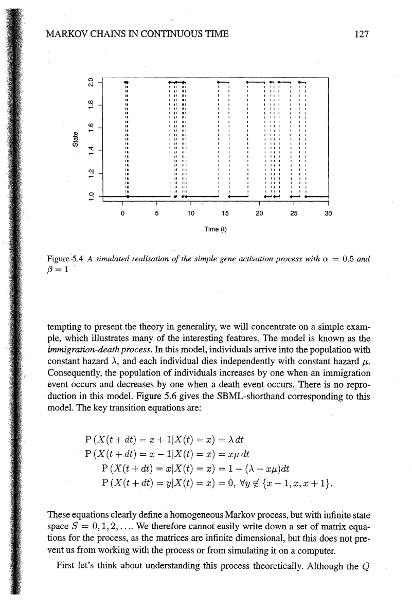
A simulated realisation
of
this process is shown
in
Figure 5.4.
5.4.2 Stochastic simulation
There are three straightforward approaches one can take to simulating this process on
a computer. The first is based on a fine time-discretisation
of
the process, similar in
spirit to the first-order Euler method for integrating ordinary differential equations.
MARKOV CHAINS IN CONTINUOUS TIME
125
Given the definition
of
the infinitesimal transition matrix
P(dt)
=I+
Qdt,
for small time steps l:.t we will have
P(t:.t)
~I+
Q t:.t.
P
(!::.
t)
can then be regarded as the transition matrix
of
a discrete time Markov chain,
and a simulated sequence
of
states at times 0, t:.t, 2 l:.t, 3 t:.t,
...
may
be
generated
in the usual way.
The above method can be easily improved by replacing the above approximation
for
P(t:.t) by its exact value
P(t:.t) = exp{Q l:.t},
provided a method for computing the matrix exponential is available. Then it does
not matter how small
l:.t is chosen to be, provided it is small enough to clearly show
the behaviour
of
the process and not
so
large that interesting transitions are "missed."
A third approach to simulation may be taken by simulating each transition event
and its corresponding time sequentially, rather than simply looking at the processes
only at times on a given lattice. Like the previous method, this gives an exact realisa-
tion
of
the process and offers the additional advantage that recording every reaction
event ensures none will
be
"missed." Such an approach is known as discrete event
simulation.
If
the process is currently in state
x,
then the
xth
row
of
Q gives the
hazards for the transition to other states. As the row sums to zero,
-qxx
gives the
combined hazard for moving away from the current state
- a discrete transition
event (note that
qxx is non-positive). So, the time to a transition event is exponential
with rate
-qxx.
When that transition event occurs, the new state will
be
random with
probabilities proportional to the xth row
of
Q (with qxx omitted). The above intuitive
explanation can
be
formalised as follows.
To
understand how to simulate the process we must consider being in state i at
time
t, and think about the probability that the next event will be in the time interval
(t + t', t +
t'
+
dt],
and will consist
of
a move to state
j.
Let this probability divided
by
dt
be
denoted by
f(t',jlt,
i), so that the probability is
f(t',Jit,
i)dt.
It
is clear
that as the Markov process is homogeneous, there will
be
no explicit dependence
on
t in this probability, but we will include it to
be
clear about exactly what we mean.
Then
f(t',jlt,i)dt
= P (Next event in (t
+t',
t +
t'
+
dt]!t,i)
x P
(jiNext
event in (t + t', t +
t'
+ dt], t,
i).
Thinking about the first term, we know that the hazards for the individual transitions
are given by the off-diagonal elements
of
the
ith
row
of
Q.
The combined hazard
is
the sum
of
these off-diagonal elements, which is
-qii
(as the row sums to zero).
Combined hazards can always
be
computed as the sum
of
hazards in this way because
the probability that two events occur in the interval (
t,
t +
dt]
is
of
order dt
2
and can
therefore be neglected. Now we know from
our
consideration
of
the exponential
distribution
as
the time to an event
of
constant hazard that the time to the next event
126 MARKOV PROCESSES
is
Exp(
-Qii),
and so the first term must
be
-Qiieq,,t'
dt. The second term is
P
(X(t
+ t' + dt) =
ji[X(t
+
t')
=
i]
n
[X(t
+
t'
+ dt)
I-
i])
P
(X(t
+
t'
+ dt) =
j!X(t
+
t')
= i) Qijdt = Qij
P(X(t+t'+dt)=f.iiX(t+t')=i)
Lk,Piqikdt
-qii
Taking the two terms together we have
f(t',jlt,i)
=
-qiieq,,t'
x
QiJ
.
-Qii
The fact that this function facto rises into the form
of
a probability density for the time
to the next event and a probability mass function for the type
of
that event means that
we can simulate the next event with the generation
of
two random variables. Note
also that there is no
j dependence in the PDF
fort'
and
not'
dependence in the PMF
for
j,
so the two random variables are independent
of
one another and hence can be
simulated independently.
It is the consideration
off
( t', j
It,
i) that leads to the standard discrete event simu-
lation algorithm which could be stated
as
follows:
1.
Initialise the process at t = 0 with initial state
i;
2.
Call the current state i. Simulate the time to the next event, t', as
an
Exp(
-Qii)
random quantity;
3.
Putt:=
t + t';
4. Simulate new state j as a discrete random quantity with PMF -Qik/qii, k
I-
i;
5. Output the
timet
and state
j;
6.
1ft<
Tmax,
return to step
2.
This particular discrete event simulation technique is known
as
the direct method. A
simpleR
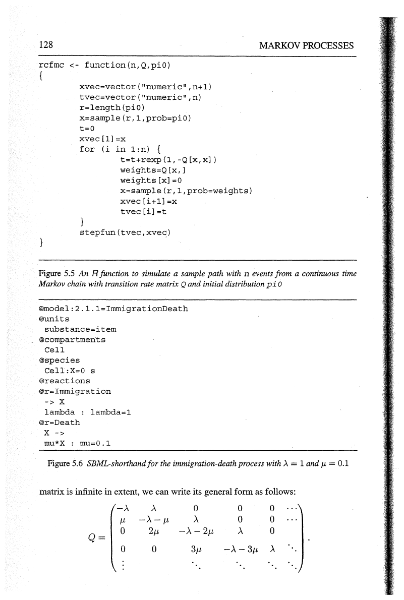
function to implement this algorithm is given in Figure 5.5. The function
returns a step-function object, which is easy to plot. Using this function, a plot similar
to Figure 5.4 can be obtained with the following command:
plot(rcfmc(20,matrix(c(-0.5,0.5,1,-1)
,ncol=2,
byrow=TRUE)
,c(l,O)))
All
of
these simulation methods give a single realisation
of
the Markov process.
Now obviously, just as one would not study a normal distribution by looking at a
single simulated value, the same is true with Markov processes. Many realisations
must be simulated in order to get a feel for the
distribution
of
values at different times.
In
the case
of
a finite number
of
states, this distribution is relatively straightforward to
compute directly without any simulation at all, but for the stochastic kinetic models
we will consider later, simulation is likely to be the only tool we have available to
us
for gaining insight into the behaviour
of
the process.
5.4.3 Countable state-space
Before moving on to thinking about continuous state spaces, it is worth spending
a little time looking at the case
of
a countably infinite state space. Rather than at-
MARKOV CHAINS
IN
CONTINUOUS TIME 127
0
..
-
_...,
~
..,..__,
.......
<.'i
"
'
"
"
'"
'
'
"
'
"
'"
'
,,
'
"l
"
'
''
'
"
" " '" "
'
"
'
"
'"
'
,,
' '
'
"
'
"
'
"
'"
'
'
~
"
'
"
"'
'
,,
"
'"
'
,,
'
"
"
'"
~
" '
"
'"
''
' '
"
'
"
'"
'
,,
' '
'
"':
"
"
'
,,
'
"
"
' '
'
"
'
"
'"
'
,,
'
"
'
"
'"
'
,,
' '
'
"l
" '
"
'"
"
'
"
"'
"
"
"
q
"
~~
..
*
+----'
..........
0
5 10 15 20 25
30
Time(!)
Figure:5.4 A simulated realisation
of
the simple gene activation process with a = 0.5 and
/3=1
tempting to present the theory in generality, we will concentrate on a simple exam-
ple, which illustrates many
of
the interesting features. The model is known as the
immigration-death process. In this model, individuals arrive into the population with
constant hazard
>.,
and each individual dies independently with constant hazard
g.
Consequently, the population
of
individuals increases by one when an immigration
event occurs and decreases by one when a death event occurs. There is no repro-
duction in this model. Figure 5.6 gives the SBML-shorthand corresponding to this
model. The key transition equations are:
P
(X(t
+
dt)
= x + 1IX(t) = x) =
>.dt
P
(X(t
+
dt)
=
x-
1jX(t) = x) =
xgdt
P
(X(t
+
dt)
= xiX(t) = x) =
1-
(>.- xg)dt
P
(X(t
+ dt) = yjX(t) = x) =
0,
Vy
rt
{x-
1,
x, x +
1}.
These equations clearly define a homogeneous Markov process, but with infinite state
spaceS
= 0, 1, 2,
....
We
therefore cannot easily write down a set
of
matrix equa-
tions for the process, as the matrices are infinite dimensional, but this does not
pre-
vent
us
from working with the process or from simulating it on a computer.
First let's think about understanding this process theoretically. Although the Q
128
rcfmc
<-
function(n,Q,piO)
xvec=vector
("numeric",
n+l)
tvec=vector
("numeric",
n)
r=length(piO)
x=sample(r,l,prob=piO)
t=O
xvec[l]=x
for
(i
in
l:n)
{
t=t+rexp(l,-Q[x,x])
weights=Q
[x,]
weights[x]=O
x=sample(r,l,prob=weights)
xvec[i+l]=x
tvec[i]=t
stepfun(tvec,xvec)
MARKOV
PROCESSES
Figure 5.5
An
R function
to
simulate a sample path with n events from a continuous time
Markov chain with transition rate matrix
Q and initial distribution
pi
0
®model:2.l.l=ImmigrationDeath
®units
substance=
item
®compartments
Cell
®species
Cell:X=O
s
®reactions
@r=Immigration
->
X
lambda
:
lambda=l
®r=Death
X
->
mu*X :
mu=O.l
Figure 5.6 SBML-shorthand
for
the immigration-death process with
>.
= 1 and
p,
= 0.1
matrix is infinite in extent, we can write its general form as follows:
->..
>..
0 0 0
J-1
-A-
J-1
A
0
0
Q=
0
2p,
-A-
2p,
A 0
0 0
3p,
-A-
3p,
A
MARKOV CHAINS IN CONTINUOUS TIME
129
Then for an infinite dimensional n = (no, n
1
,
n
2
,
...
) we can solve
nQ
= 0 to get
the 'stationary distribution one equation at a time, expressing each
nk
in terms
of
no
to
find the general form
)..k
nk
=
-k
1
k no, k =
1,
2,
....
·11
But these are terms in the expansion
of
n
0
e>-l
~',
and so imposing the unit-sum con-
straint we get
no = e-AIJL giving the general solution
This is easily recognised as the PMF
of
a Poisson random quantity with mean
>.j
p,
(Section 3.6). Hence, the stationary distribution
of
this process is Poisson with mean
>.ill·
We_can
also simulate realisations
of
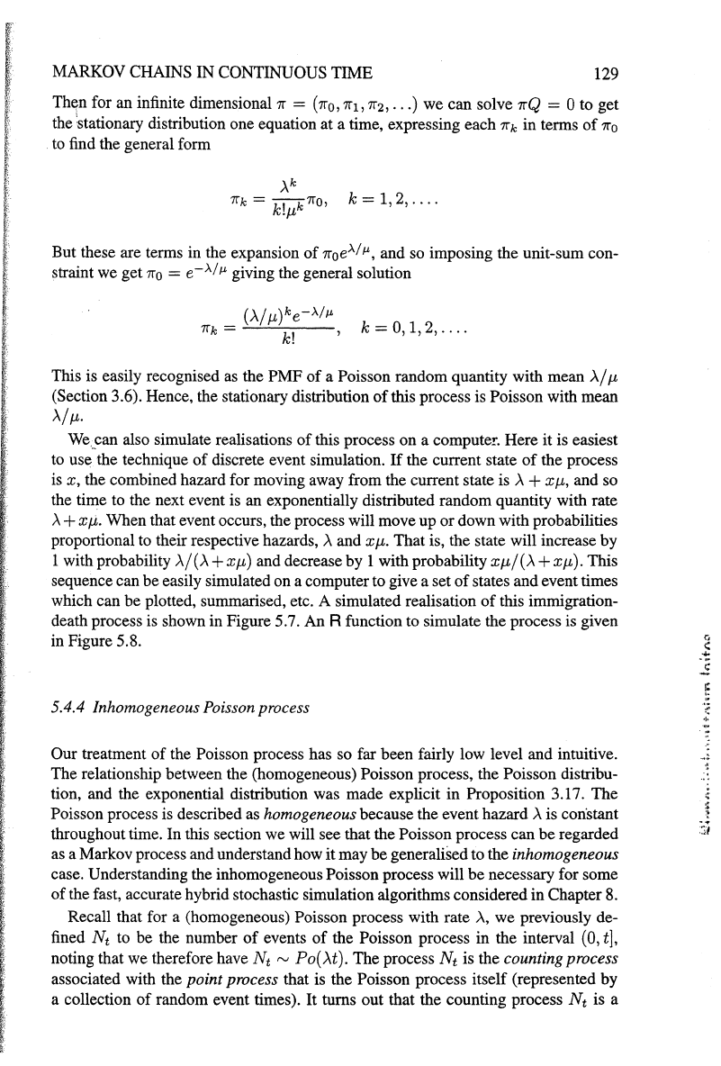
this process on a computer. Here it is easiest
to
use the technique
of
discrete event simulation.
If
the current state
of
the process
is
x, the combined hazard for moving away from the current state is
)..
+
XJl,
and so
the time
to
the next event is an exponentially distributed random quantity with rate
>.
+
XJ1.
When that event occurs, the process will move up
or
down with probabilities
proportional to their respective
hazards,).. and
xp,.
That is, the state will increase by
1 with probability
>.j(>.+xJl) and decrease by 1 withprobabilityxJ1/(>.+xJ1). This
sequence can be easily simulated on a computer to give a set
of
states and event times
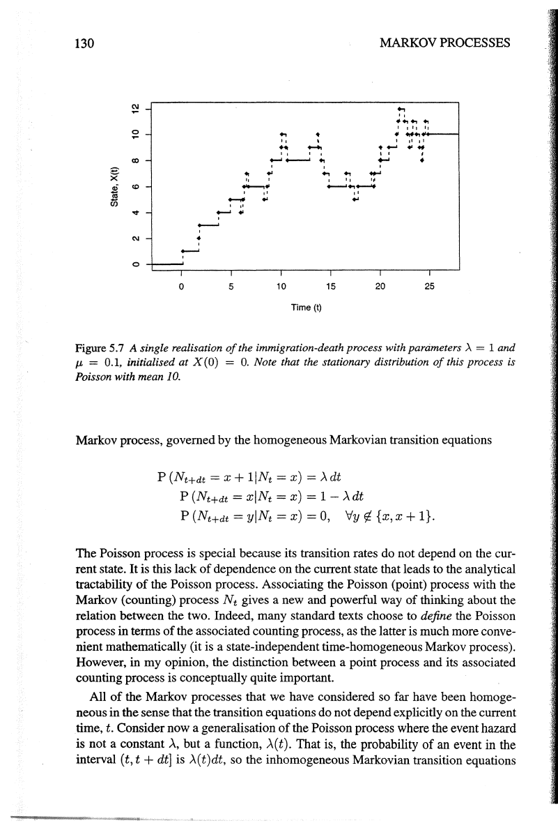
which can be plotted, summarised, etc. A simulated realisation
of
this immigration-
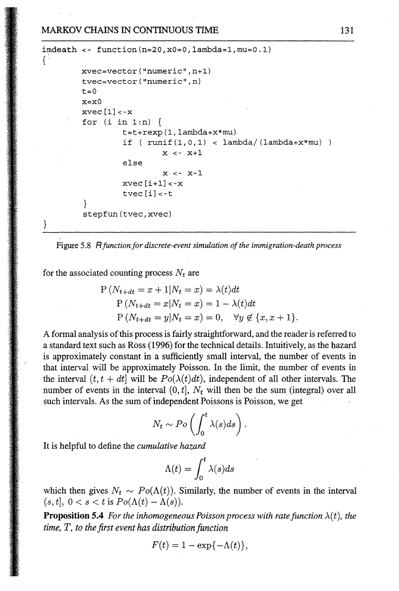
death process is shown in Figure 5.7. An R function to simulate the process is given
in Figure 5.8.
5.4.4 Inhomogeneous Poisson process
Our treatment
of
the Poisson process has so far been fairly low level and intuitive.
The relationship between the (homogeneous) Poisson process, the Poisson distribu-
tion, and the exponential distribution was made explicit in Proposition 3.17. The
Poisson process is described as
homogeneous because the event hazard
)..
is constant
throughout time. In this section we will see that the Poisson process can be regarded
as a Markov process and understand how
it
may be generalised to the inhomogeneous
case. Understanding the inhomogeneous Poisson process will be necessary for some
of
the fast, accurate hybrid stochastic simulation algorithms considered in Chapter 8.
Recall that for a (homogeneous) Poisson process with rate
>.,
we previously de-
fined
Nt
to
be the number
of
events
of
the Poisson process in the interval (0,
t],
noting that we therefore have
Nt
"'
Po(>..t). The process
Nt
is the counting process
associated with the point process that is the Poisson process itself (represented by
a collection
of
random event times). It turns out that the counting process
Nt
is a
r,
<:
.:";
..:
E
.::
130
~
0
"'
~
~
<0
(/)
'<!"
C\1
0
0
..,
,,
...
•
.
.....
.....;~~
MARKOV PROCESSES
...
,,
.
.,
.,
.,
~~~~
I
tl
tl
• ...,.a
..
.,
I'
I
- .
~
~
~
.,
*""
1 I 1
I~
-..
..
..............
-
'
,,
,,
-
..
...
'
,,
.........
5
10
15
20
25
Time(!)
Figure 5.7 A single realisation
of
the immigration-death process with parameters
.A
= 1 and
p.
= 0.1, initialised
at
X(O) =
0.
Note that the stationary distribution
of
this process is
Poisson with mean
10.
Markov process, governed
by
the homogeneous Markovian transition equations
P (Nt+dt = x
+liNt=
x)
=
>..dt
P (Nt+dt =
x!Nt
=
x)
=
1-
)..dt
P (Nt+dt =
yjNt
=
x)
=
0,
Vy
r/:
{x,x
+ 1}.
The
Poisson process is special because its transition rates do not depend
on
the cur-
rent
state.
It
is this
lack
of
dependence
on
the current state that leads to the analytical
tractability
of
the Poisson process. Associating the Poisson (point) process with the
Markov (counting) process
Nt
gives a new and powerful way
of
thinking about the
relation between the two. Indeed, many standard texts choose to define the
Poisson
process
in
terms
of
the associated counting process, as the latter is much more conve-
nient mathematically (it is a state-independent time-homogeneous Markov process).
However,
in
my
opinion, the distinction between a point process and its associated
counting process is conceptually quite important.
All
of
the Markov processes that
we
have considered so far have been homoge-
neous in the sense that the transition equations do not depend explicitly
on
the current
time,
t. Consider now a generalisation
of
the Poisson process where the event hazard
is
not
a constant>.., but a function,
>..(t).
That
is, the probability
of
an event
in
the
interval
(t, t + dt] is
>..(t)dt,
so the inhomogeneous Markovian transition equations
MARKOV CHAINS
iN
CONTINUOUS TIME
imdeath
<-
function(n=20,x0=0,lambda=1,mu=0.1)
(
xvec=vector
("numeric",
n+1)
tvec=vector
("numeric",
n)
t=O
X=XO
xvec[1]<-X
for
(i
in
1
:n)
t=t+rexp(1,lambda+x*mu)
if
(
runif(1,0,1)
<
lambda/(lambda+x*mu)
X
<-
X+1
else
x
<-
x-1
xvec[i+1]<-x
tvec[i]<-t
stepfun(tvec,xvec)
131
Figure
5.8
R function
for
discrete-event simulation
of
the immigration-death process
for the associated counting process
Nt
are
P (Nt+dt = x
+liNt=
x)
=
>-.(t)dt
P (Nt+dt =
xiNt
=
x)
=
1-
>-.(t)dt
P (Nt+dt = y!Nt =
x)
=
0,
'Vy
¢
{x,x
+
1}.
A formal analysis
of
this process is fairly straightforward, and the reader is referred to
a standard text such as Ross ( 1996) for the technical details. Intuitively, as the hazard
is approximately constant
in
a sufficiently small interval, the number
of
events in
that interval will be approximately
Poisson. In the limit, the number
of
events in
the interval
(t, t +
dt}
will be
Po(>-.(t)dt),
independent
of
all other intervals. The
number
of
events in the interval
(0,
t],
Nt
will then
be
the sum (integral) over all
such intervals. As
the sum
of
independent Poissons is Poisson, we get
Nt
"'Po
(lot
>-.(s)ds).
It
is helpful to define the cumulative hazard
A(t)
=lot
>-.(s)ds
which then gives
Nt
"'
Po(A(t)). Similarly, the number
of
events
in
the interval
(s, t], 0 < s
<tis
Po(A(t)-
A(s)).
Proposition 5.4
For
the
inhomogeneous Poisson process with
rate
function
>-.(t),
the
time,
T,
to
the
first
event
has
distribution
function
F(t) =
1-
exp{
-A(t)},
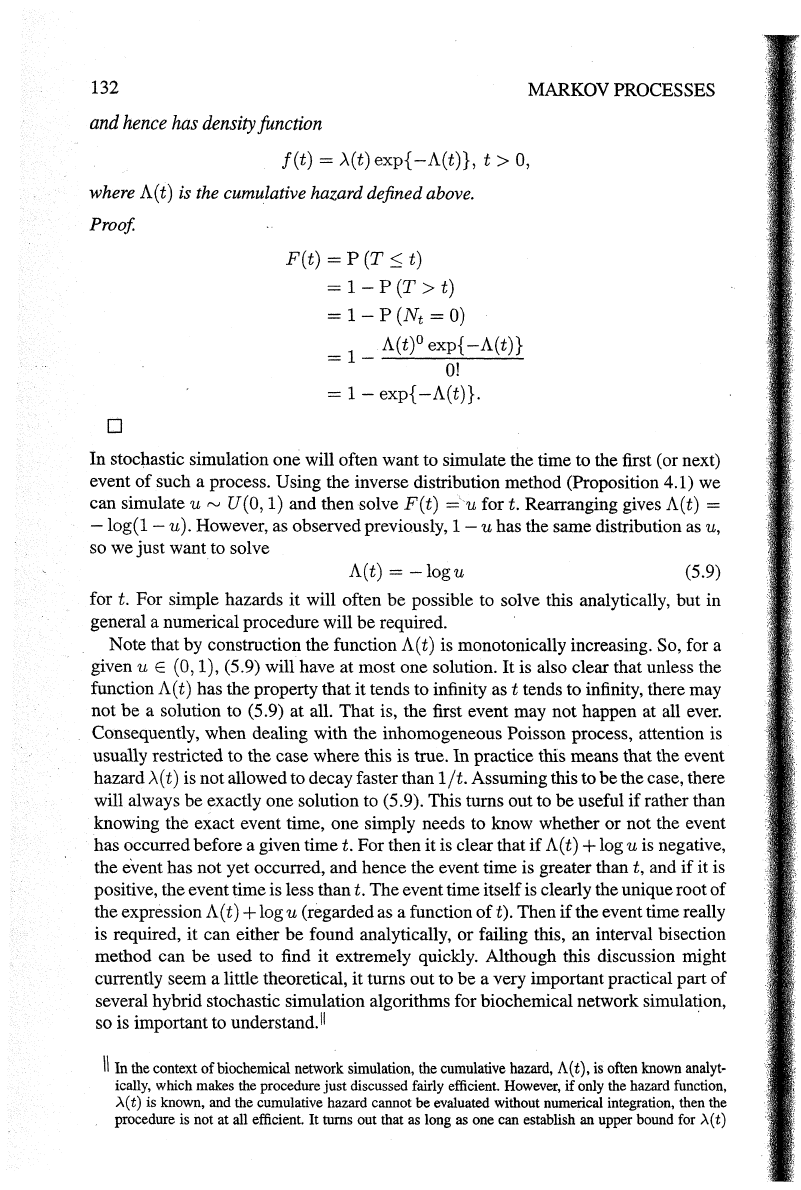
132
MARKOV PROCESSES
and
hence
has
density
function
f(t)
=
.A(t)
exp{
-A(t)},
t > 0,
where A(t) is the cumulative hazard defined above.
Proof
D
F(t)
= P (T
~
t)
=
1-
P (T > t)
=
1-
P (Nt =
0)
=
1
__
A..:....(t'-)
0
_ex-=p-"'"{_-A_(.:....;t)'""-}
0!
=
1-
exp{
-A(t)}.
In stochastic simulation one will often want to simulate the time to the first (or next)
event
of
such a process. Using the inverse distribution method (Proposition 4.1) we
can simulate
u
~
U(O,
1) and then solve
F(t)
= u
fort.
Rearranging gives A(t) =
-log(1-
u). However, as observed previously,
1-
u has the same distribution as u,
so we just want to solve
A(t)
=
-logu
(5.9)
for
t.
For simple hazards it will often be possible to solve this analytically, but in
general a numerical procedure will be required.
Note that by construction the function A(t) is monotonically increasing.
So, for a
given
u E (0, 1), (5.9) will have at most one solution.
It
is also clear that unless the
function A(
t)
has the property that it tends to infinity as t tends to infinity, there may
not
be
a solution to (5.9) at all. That is, the first event may not happen at all ever.
Consequently, when dealing with the inhomogeneous
Poisson process, attention is
usually restricted to the case where this is true.
In
practice this means that the event
hazard
.A(t)
is not allowed to decay faster than
1/t.
Assuming this to be the case, there
will always be exactly one solution to (5.9). This turns out to be useful
if
rather than
knowing the exact event time, one simply needs to know whether or not the event
has occurred before a given
timet.
For then
itis
clear that
if
A(
t)
+log
u is negative,
the
event has not yet occurred, and hence the event time is greater than t, and
if
it is
positive, the event time is less than
t. The event time itself is clearly the unique root
of
the expression A(
t)
+log
u (regarded as a function
oft).
Then
if
the event time really
is required, it can either be found analytically, or failing this, an interval bisection
method can be used to find
it
extremely quickly. Although this discussion might
currently seem a little theoretical, it turns out to be a very important practical part
of
several hybrid stochastic simulation algorithms for biochemical network simulation,
so is important to understand.
II
·
II
In the context
of
biochemical network simulation, the cumulative hazard,
A(t),
is often known analyt-
ically, which makes the procedure
just
discussed fairly efficient However,
if
only the hazard function,
;>.(
t)
is known, and the cumulative hazard cannot
be
evaluated without numerical integration, then the
procedure is not
at
all efficient.
It
turns out that as long as one can establish an upper bound for
;>.(t)
DIFFUSION PROCESSES
133
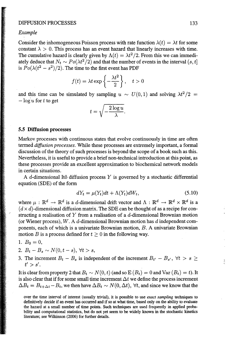
Example
Consider the inhomogeneous Poisson process with rate function
.A(t)
=.At
for some
constant
.A
> 0. This process has an event hazard that linearly increases with time.
The cumulative hazard is clearly given by A(t)
=
.At
2
/2.
From
this
we
can immedi-
ately deduce that
Nt
""'
Po(.At2
/2)
and that the number
of
events in the interval (s,
t]
is
Po(.A(t
2
- s
2
)/2).
The
time to the first event has
PDF
f(t)=.Atexp{-).~
2
},
t>O
and this time can
be
simulated by sampling u
""'
U(O,
1) and solving
.At2
/2
-log'u
fort
to get
t =
J-
2l:gu_
5.5 Diffusion processes
Markov processes with continuous states that evolve continuously
in
time are often
termed
diffusion processes. While these processes are extremely important, a formal
discussion
of
the theory
of
such processes is beyond the scope
of
a book such as this.
Nevertheless, it is useful to provide a brief non-technical introduction at this point, as
these processes provide an excellent approximation to biochemical network models
in certain situations.
A d-dimensional
Ito
diffusion process Y is governed
by
a stochastic differential
equation (SDE)
of
the form
dyt
=
J.L(Yt)dt
+ A(yt)dWt,
(5.10)
where
JL
:
JRd
-+
JRd
is a d-dimensional drift vector and A :
JRd
-+
JRd
x
JRd
is a
( d x d)-dimensional diffusion matrix. The SDE can
be
thought
of
as a recipe for con-
structing a realisation
of
Y from a realisation
of
a d-dimensional Brownian motion
(or Wiener process),
W. A d-dimensional Brownian motion has d independent com-
ponents, each
of
which is a univariate Brownian motion, B. A univariate Brownian
motion
B is a process defined for t
:2:
0 in the following way.
1.
Eo=
0,
2.
Bt-
Bs ""'N(O,
t-
s),
Vt
>
s,
3.
The increment
Bt
- Bs is independent
of
the increment Bt' - Bs',
Vt
> s
:2:
t' >
s'.
It
is clear from property 2 that
Bt
""'
N(O, t) (and so E (Bt) = 0 and
Var
(Bt) = t).
It
is also clear that
if
for some small time increment
t:J.t
we define the process increment
.6.Bt =
Bt+At-
Bt, we then have
!::J.Bt
,.._,
N(O,
t:J.t),
Vt, and since
we
know that the
over the time interval of interest (usually trivial), it
is
possible to use exact sampling techniques
to
definitively decide
if
an
event has occurred and if so at what time, based only on the ability to evaluate
the hazard
at
a small number
of
time points. Such techniques are used frequently in applied proba-
bility
and
computational statistics, but
do
not
yet seem to be widely known in the stochastic kinetics
literature; see Wilkinson
(2006) for further details.
