Wilkinson D.J. Stochastic Modelling for Systems Biology
Подождите немного. Документ загружается.

74
PROBABILITY MODELS
sample mean
X,
then
2
E(.X)
=f.L
and
Var(.X)
=
~-
n
Proof The result follows immediately from Propositions 3.5 and 3.6. D
Lemma 3.7 (Markov's inequality)
If
X
::::
0 is a non-negative random quantity
with finite expectation
E (X) =
f.L
we have
P(X::::a):::;t!:,
Va>O.
a
Proof Note that this result is true for arbitrary non-negative random quantities, but
we present here the proof for the continuous case.
D
f.L
E(X)
a a
=
~
roo
~f(x)
dx
a
lo
=
roo~
f(x)dx
lo
a
:::=::
1
00
~
f(x)dx
a a
:::=::
1
00
'3:.
f(x)dx
a a
=
1=
f(x)dx
= P
(X
:2:
a).
Lemma 3.8 (Chebyshev's inequality)
If
X is a· random quantity with finite mean
E (X) =
f.L
and variance Var
(X)=
a
2
we have
1
P
(JX-
f.LI
< ka)
::::
1-
k
2
,
Vk
>
o.
Proof
Since
(X
-
f.L
)2
is positive with expectation a
2
,
Markov's inequality gives
IJ2
P
([X-
f.L]
2
:::=::a)::::;-.
a
Putting a = k
2
a
2
then gives
D
p
([X-
f.L]2
::::
k2a2)
::::;
:2
1
'*
P(JX-
f.LI::::
ka)::::;
k
2
1
'*
P
(JX-
f.Li
< ka)
;:::
1-
k
2
.
\
THE
cinFORM
DISTRIBUTION
75
We
are now in a position to state the main result.
Proposition
3.14
(weak
law
of
large
numbers,
WLLN)
For X with finite mean
E
(X)·=
p,
and
variance Var (X) =
(]'
2
,
if
X
1
,
X
2
,
...
,
Xn
is an independent sam-
ple from X used to form the sample mean
X,
we have
- (]'2 n
P
(IX-
J.£1
<c)
~
1-
-
2
--+
1,
Vc
>
o.
nc
oo
In other words, the WLLN states that no matter how small one chooses the positive
constant
c,
the probability that X is within a distance c
of
p,
tends to 1 as the sample
size
n increases. This is a precise sense
in
which the sample mean "converges" to the
expectation.
Proof. Using Lemmas 3.6 and 3.8
we
have
Substihiting k = E
.Jii
/
(j
gives the result. D
This result is known as the weak law, as there is a corresponding strong law, which
we state without proof.
Proposition
3.15
(strong
law
oflarge
nnmbers,
SLLN)
For X with finite mean E
(X)
=
p,
and variance Var
(X)=
(]'
2
,
if
X
1
,
X2,
...
,
Xn
is an independent sample from X
used to form the sample mean
X,
we have
3.8
The
uniform
distribution
Now that
we
understand the basic properties
of
continuous random quantities,
we
can
look at some
of
the important standard continuous probability models.
The
simplest
of
these is the uniform distribution. This distribution turns out to
be
central to the
theory
of
stochastic simulation that will be developed in the next chapter.
The random quantity
X has a uniform distribution over the range [a,
b],
written
if
the
PDF
is given by
X"'
U(a,
b)
fx(x)={b~a'
0,
a~
x
~
b,
otherwise.
76
PROBABILITY
MODELS
PDFforX-U(0,1)
CDF
for
X-
U(0,1)
~
~
~ ~
~ ~
;?
~
~ ~
~
~
:l
0
-{),5
0.0 0.5 1.0
1.5
-{),5
0.0 0.5
1.0
1.5
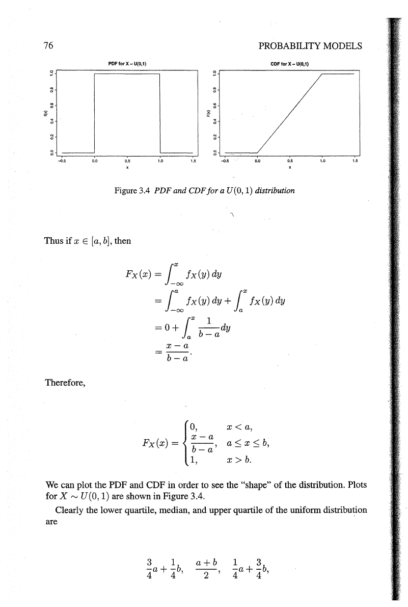
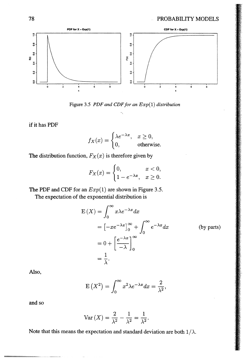
Figure 3.4
PDF
and CDF
for
a U(O, 1) distribution
Thus
if
x E [a,
b],
then
Fx(x)
=
j_xoo
fx(y)
dy
=
j_aoo
fx(y)
dy +
1x
fx(y)
dy
1
x 1
= 0 + a
b-
ady
x-a
=
b-a·
Therefore,
{
0,
x
<a,
x-a
Fx(x)
= b
_a,
aS
x S
b,
1,
X>
b.
We can plot the PDF and CDF
in
order to see the "shape"
of
the distribution. Plots
for
X~
U(O,
1) are shown in Figure 3.4.
Clearly the lower quartile, median,
and upper quartile
of
the uniform distribution
are
a+b
-2-,
THE
EXPONENTIAL DISTRIBUTION
respectively. The expectation
of
a uniform random quantity is
E
(X)
=I:
x
fx(x)
dx
=
[~
x
fx(x)
dx
+
1b
x
fx(x)
dx
+
loo
x
fx(x)
dx
= 0 +
1b
b : a
dx
+ 0
=
[2(bx~
a)J:
a+b
2
We
can also calculate the variance
of
X.
First we calculate E
(X
2
)
as follows:
Now,
l
b 2
E (
X2)
= a b
~
a
dx
b
2
+
ab+
a
2
3
Var
(X)=
E
(X
2
) -
E
(X)
2
b
2
+ab+a
2
(a+b)2
3 4
(b-
a)
2
12
77
The uniform distribution is too simple to realistically model actual experimental data,
but is very useful for computer simulation, as random quantities from many different
distributions can be obtained from
U
(0,
1) random quantities.
3.9 The exponential distribution
For reasons still to be explored,
it
turns
out
that the exponential distribution is the
most important continuous distribution in the theory
of
discrete-event stochastic sim-
ulation.
It
is therefore vital to have a good understanding
of
this distribution and its
many useful properties. We will begin by introducing this distribution
in the abstract,
but we will then go on to see why it arises so naturally by exploring its relationship
with the
Poisson process.
The random variable X has an exponential distribution with parameter
>.
> 0,
written
X,....,
Exp(>.)
78
PROBABILITY
MODELS
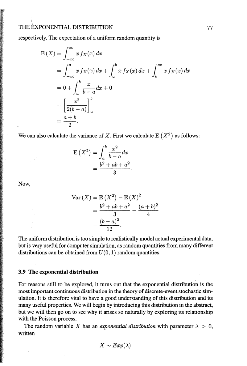
PDF for
X-
Exp{1)
CDF for
X-
Exp(1)
:0
0
~
if
;;
~
~
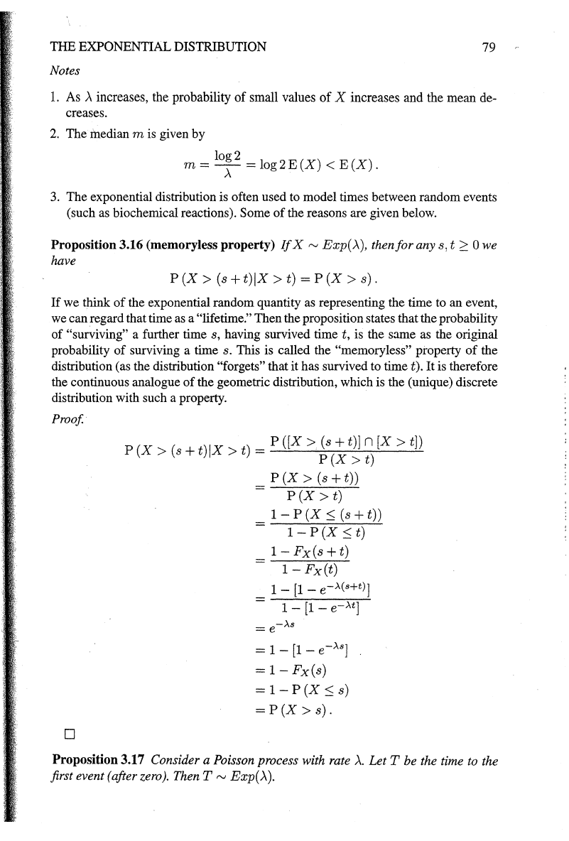
Figure 3.5
PDF
and CDF
for
an
Exp(l)
distribution
if
it has PDF
fx(x)
=
{.>..e->-x,
x
::2:
0,.
0, otherwise.
The distribution function,
F x ( x) is therefore given by
{
0,
X<
0,
Fx(x)
=
1-
e->-x,
X
::2:0.
The PDF and CDF for an Exp(1) are shown in Figure 3.5.
The expectation
of
the exponential distribution is
(by parts)
Also,
and so
2 1 1
Var(X) = .>,.2-
.>,.2
=
.>,.2"
Note that this means the expectation and standard deviation are both 1 j
.>...
THE EXPONENTIAL DISTRIBUTION
79
Notes
1.
As A increases, the probability
of
small values
of
X increases and the mean de-
creases.
2.
The median m
is
given by
log2
m
=-.A-=
log2E(X)
<
E(X).
3.
The exponential distribution is often used
to
model times between random events
(such as biochemical reactions). Some
of
the reasons are given below.
Proposition 3.16 (memoryless property)
If
X""
Exp(.A), then
for
any s, t
2:
0 we
have
P
(X>
(s +
t)IX
> t) = P
(X>
s).
If
we think
of
the exponential random quantity as representing the time
to
an event,
we can regard that time as a
"lifetime." Then the proposition states that the probability
of
"surviving" a further time
s,
having survived time
t,
is the same as the original
probability
of
surviving a time s. This is called the "memoryless" property
of
the
distribution (as the distribution
"forgets" that it has survived to time
t).lt
is therefore
the continuous analogue
of
the geometric distribution, which is the (unique) discrete
distribution with such a property.
Proof.
0
P
(X
(
)IX
)
= P
([X>
(s
+ t)] n
[X>
t])
> s + t > t p
(X
>
t)
P(X
>
(s+t))
P(X
> t)
1-
P
(X
:S
(s + t))
1-
P
(X
:S
t)
1-Fx(s+t)
1-
Fx(t)
1 -
[1
- e->-(s+t)]
1-
[1-
e->-t]
=
e->-s
= 1 -
[1
-
e->-s]
=
1-
Fx(s)
=1-P(X:Ss)
=P(X>s).
Proposition 3.17 Consider a Poisson process with rate
A.
Let T be the time to the
first event (after zero). Then
T
""
Exp(
A).
80
PROBABILITY MODELS
Proof.
Let
Nt
be the number
of
events in the interval
(0,
t]
(for given fixed t > 0).
We have seen previously that (by definition)
Nt
rv
Po()..t). Consider the CDF
ofT,
Fr(t)
= P
(T::;
t)
=
1-
P
(T
> t)
=
1-
P(Nt
=
0)
()..t)Oe->.t
= 1 -
-'--'-.--
0!
=1-e->-t.
This is the distribution function
of
an Exp()..) random quantity, and
soT"'
Exp(>..).
D '
So the time to the first event
of
a Poisson process is an exponential random vari-
able. But then using the independence properties
of
the Poisson process, it should be
reasonably clear that the time between any two such events has the same exponential
distribution. Thus the times between events
of
the Poisson process are exponential.
There is another way
of
thinking about the Poisson process that this result makes
clear. For an infinitesimally small time interval
dt we have
P (T::; dt) =
1-
e-)..dt
=
1-
(1-
)..dt) =
>..dt,
and due to the independence property
of
the Poisson process, this is the probability
for any time interval
oflength
dt. The Poisson process can therefore be thought
of
as
a process with constant event "hazard"
>..,
where the "hazard" is essentially a measure
of
"event density" on the time axis. The exponential distribution with parameter
>..
can therefore also be reinterpreted as the time to an event
of
constant hazard
>...
The two properties above are probably the most fundamental. However, there are
several other properties that we will require
of
the exponential distribution when we
come to use it to simulate discrete stochastic models
of
biochemical networks, and
so they are mentioned here for future reference. The first describes the distribution
of
the minimum
of
a collection
of
independent exponential random quantities.
Proposition 3.18
If
Xi
"'
Exp(>...i),
i = 1,
2,
...
, n, are independent random vari-
ables, then
n-
Xo
=min{
Xi}
rv
Exp(>..o),
where
Ao
=
I>i·
t
i=l
THE
EXPONENTIAL DISTRIBUTION
Proof. First note that for X
rv
Exp()..) we have p
(X
>
X)
=
e-
AX. Then
P
(Xo
> x) = P
(~in{
Xi}>
x)
= P
([X1
>
x]
n
[X2
>
x]
n · · · n
[Xn
> x])
n
i=l
i=l
SoP
(Xo
:::;
x) =
1-
e->-ox
and hence X
0
rv
Exp(:>..
0
).
0
The next lemma is for the following proposition.
81
Lemma 3.9 Suppose that X
rv
Exp(:>..)
andY
rv
Exp(p,) are independent random
variables. Then
Proof.
0
)..
P(X
<
Y)
=
-,-.
/\+f.L
p
(X
<
Y)
= 1
00
p
(X
<
YIY
= y)
f(y)
dy
=
1oo
P(X
<
y)f(y)dy
=
1oo
(1
-
e-AY)p,e-1-'Y
dy
)..
:>..+p,
(Proposition 3.11)
This next result gives the likelihood
of
a particular exponential random quantity
of
an independent collection being the smallest.
Proposition 3.19
If
Xi
rv
Exp(;>..i),
i =
1,
2,
...
, n are independent random vari-
ables, let
j be the index
of
the smallest
of
the Xi. Then j is a discrete random variable
withPMF
Proof.
n
i = 1, 2,
...
,
n,
where
>-o
=
2.::::
>.i.
i=l
1r·
= P
(x·
<
min{x})
J J
i#j
•
=
P(Xi
<
Y)
82
PROBABILITY
MODELS
(by
the lemma)
0
This final result is a trivial consequence
of
Proposition 3.12.
Proposition 3.20 Consider X
rv
Exp(:>..).
Then
for
a >
0,
y =
aX
has distribu-
tion
Y "'Exp(:>..ja).
3.10 The normal/Gaussian distribution
3.1
0.1 Definition
and
properties
Another fundamental distribution
in
probability theory is the normal
or
Gaussian
distribution.
It
turns
out
that sums
of
random
quantities often approximately fol-
low a normal distribution.
Since
the
change
of
state
of
a biochemical network
can
sometimes
be
represented
as
a
sum
of
random quantities,
it
turns out that normal
distributions are useful in this context.
Definition 3.15 A random quantity X has a normal distribution with parameters
p,
and
a
2
,
written
if
it
has probability density function
fx(x)
=
--
exp
--
--
,
1 {
l(x-p,)
2
}
a...!2if
2 a
-oo
< x <
oo,
fora>
0.
Note
that
fx(x)
is symmetric about x =
p,,
and
so
(provided the density integrates
to
1 ), the median
of
the
distribution will
be
p,.
Checking that the density integrates
·to
1 requires the computation
of
a difficult integral. However,
it
follows directly from
the known
"Gaussian" integral
1
00
-a:z:
2
dx
If
e =
-,
-oo
a
a>O,
THE NORMAL/GAUSSIAN DISTRIBUTION
83
PDFforX-N(0,1)
CDF
for X~
N{0,1)
:0
~
~
~
~
~
~
_,
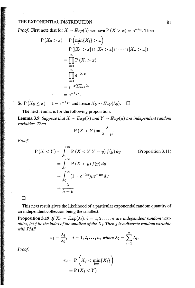
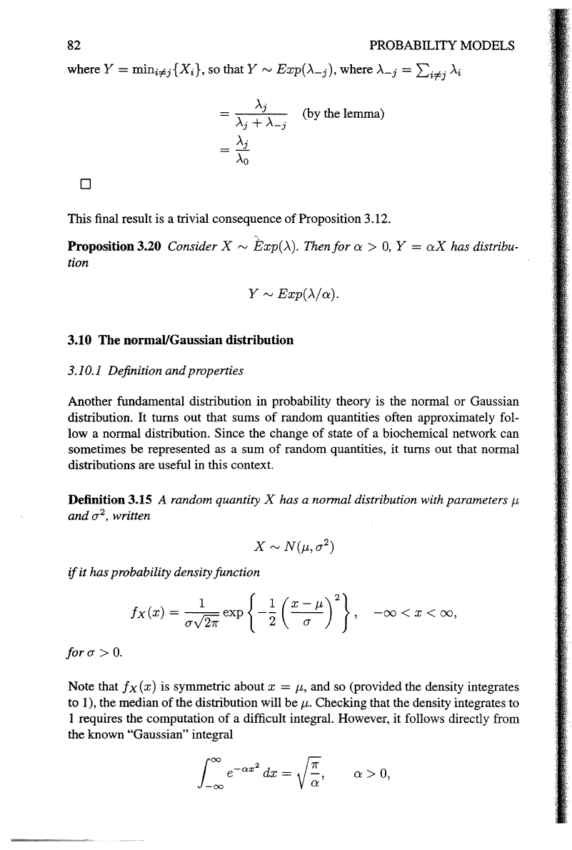
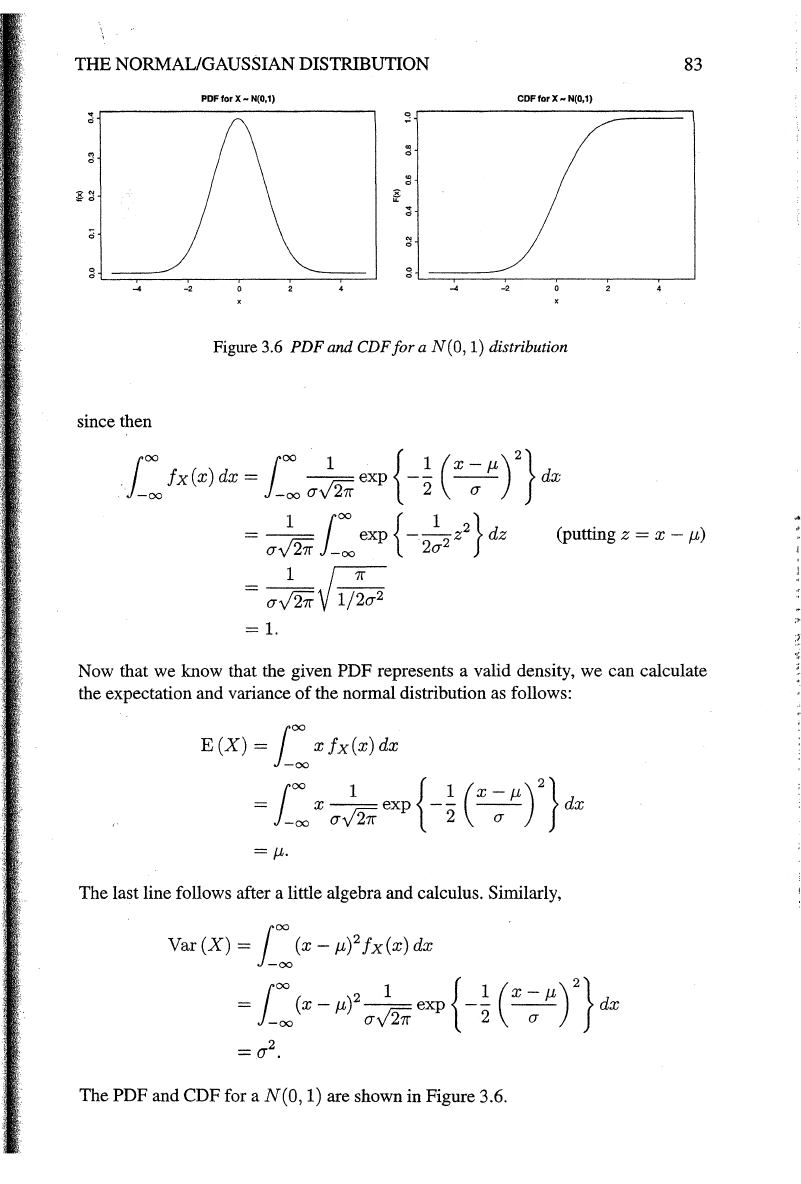
Figure 3.6
PDF
and CDF
for
a N(O, 1) distribution
since then
j
oo
joo
1 { 1
(X
p,)
2
}
.
fx(x)dx=
r.:cexp
--
--
dx
-oo -oo
tTy
27r
2 tT
(putting z = x -
p,)
Now that we know that the given PDF represents a valid density, we can calculate
the expectation and variance
of
the normal distribution as follows:
E(X)
=I:
xfx(x)dx
j
oo
1 { 1
(x-p,)
2
}
=
x--exp
--
--
dx
-00
(JJ27r
2
(J
=
p,.
The last line follows after a little algebra and calculus. Similarly,
Var
(X)
=I:
(x-
p,)
2
fx(x)
dx
=
joo
(x-
p,?-
1
exp
{-~
(x-
p,)
2
}
dx
-oo
(JJ27r
2
tT
=
az.
The PDF and CDF for a N(O, 1) are shown in Figure 3.6.