Vidakovic B. Statistics for Bioengineering Sciences: With Matlab and WinBugs Support

Подождите немного. Документ загружается.

Chapter 18

Inference for Censored Data and Survival

Analysis

The ﬁrst condition of progress is the removal of censorship.

– George Bernard Shaw

WHAT IS COVERED IN THIS CHAPTER

• Parametric Models for Time-to-Event Data

• Kaplan–Meier Estimator

• Cox Proportional Hazards Model

• Bayesian Approaches

18.1 Introduction

Survival analysis models the survival times of a group of subjects (usually

shows how many of the subjects are “alive” or survive over time.

ology is the presence of censored observations; in addition, some subjects may

have left the study and may be lost to follow-up. Such subjects were known to

have survived for some amount of time (up until the time we last saw them),

but we do not know how much longer they might ultimately have survived.

What makes survival analysis different from the standard regression method-

B. Vidakovic, Statistics for Bioengineering Sciences: With MATLAB and WinBUGS Support,

Springer Texts in Statistics, DOI 10.1007/978-1-4614-0394-4_18,

701

with some kind of medical condition) and generates a survival curve, which

Several methods have been developed for using this “at least this long” infor-

702 18 Inference for Censored Data and Survival Analysis

mation to ﬁnding unbiased survival curve estimates, the most popular being

the nonparametric method of Kaplan and Meier.

An observation is said to be censored if we know only that it is less than

(or greater than) a certain known value. For instance, in clinical trials, one

could be interested in patients’ survival times. Survival time is deﬁned as the

length of time between diagnosis and death, although other “start” events

(such as surgery), and other “end” events (such as relapse of disease, increase

in tumor size beyond a particular threshold, rejection of a transplant, etc.) are

commonly used. Because of many constraints, trials cannot be run until the

endpoints are observed for all patients. Just because for a particular subject

the time to endpoint is not fully observed, partial information is still avail-

able: the patient survived up to the end of the observational period, and this

should be incorporated into the analysis. Such observations are called right

censored. Observations can also be left censored, for example, an assay may

have a detection threshold. In order to utilize information contained in cen-

sored observations, special methods of analysis are required.

Biomedical engineers are often interested in the reliability of medical de-

vices, and most of the methodology from survival analysis is applicable in

device reliability analyses. There are of course important differences. In the

reliability of multicomponent systems an important aspect is optimization of

the number and position of components. Analogous considerations with or-

gans or parts of organs as components in living systems (animals or humans)

are impossible. Methods such as “accelerated life testing” commonly used in

engineering reliability are inappropriate when dealing with human subjects.

However, in comparing the lifetimes of subjects in clinical trials involving

different treatments (humans, animals) or different engineering interventions

(systems, devices), the methodology that deals with censored observations is

shared.

18.2 Deﬁnitions

Let T be a random variable with CDF F(t) representing a lifetime. The sur-

vival (or survivor) function is the tail probability for T, i.e., S(t)

=1−F(t), t >0.

The function S(t) gives the probability of surviving up to time t, that is,

S(t) =P(T > t).

The hazard function or hazard rate is deﬁned as

18.2 Deﬁnitions 703

h(t) =

f (t)

S(t)

f (t)

1 −F(t)

when T has a density f (t). Note that S

(t) =−f (t). It is insightful to represent

h(t) in limit terms,

S(t)

−S(t +∆t)

∆t

S(t)

F(t +∆t)−F(t)

∆t

S(t)

(t < T ≤ t +∆t)

∆t P(T > t)

(T ≤ t +∆t|T >t)

∆t

when

∆t → 0. It represents “an instantaneous” probability that an event that

was not observed up to time t will be observed before t

+∆t, when ∆t →0.

Cumulative hazard is deﬁned as H(t)

h(s)ds. Both hazard and cu-

mulative hazard uniquely determine the distribution of lifetime F, F(t)

1 −exp{−

h(s)ds}, i.e., F(t) = 1 −exp{−H(t)}. Cumulative hazard can also be

connected to the survival function as H(t)

=−log S(t), or

S(t)

=exp{−H(t)}. (18.1)

Example 18.1. The hazard function for an exponential distribution with den-

sity f (t)

=λe

−λt

, t ≥0,λ >0 is constant in time, h(t) =λ.

Example 18.2. The hazard rate for a one-parameter Weibull distribution with

CDF F(t)

=1 −exp{−t

} and density f (t) =γt

(γ−1)

exp{−t

}, t ≥0, γ >0 is h(t) =

γt

γ−1

. The parameter γ is called a shape parameter. Depending on the “shape

parameter,”

γ, the hazard function h(t) could model various types of survival

analyses.

The two-parameter version of Weibull is used more frequently. It is deﬁned

as F(t)

=1−exp{−λt

}, with density f (t) =λγt

(γ−1)

exp{−λt

}, t ≥0, γ >0,λ >0.

The parameter

λ is called a “rate” parameter. In this case h(t) =λγt

Two important summaries in the parametric case (where the survival dis-

tribution is speciﬁed up to a parameter) are mean residual life (mrl) and me-

dian life, deﬁned respectively as

704 18 Inference for Censored Data and Survival Analysis

mrl(t) =

∞

S(x)dx

S(t)

0.5

: S(t

0.5

) =0.5.

Example 18.3. For an exponential lifetime, the expected lifetime and mrl coin-

cide. Indeed,

ET =1/λ, while

mrl(t)

∞

−λx

−λt

At ﬁrst glance this looks like a paradox, the expected total lifetime

ET is

equal to the residual lifetime mrt(t) irrespective of t. This is an example of

the “inspection paradox” that follows from the memoryless property of the ex-

ponential distribution. The median lifetime of an exponential distribution is

0.5

=(log2)/λ.

In MATLAB, dfittool, normfit, wblfit, and other commands for ﬁtting

parametric distributions can be applied to censored data by specifying the cen-

soring vector at input.

18.3 Inference with Censored Observations

We will consider the case of right-censored data (the most common type of

censoring) and two approaches: a parametric approach, in which the survival

function S(t) would have a speciﬁc functional form, and a nonparametric ap-

proach, in which no such functional form is assumed.

18.3.1 Parametric Approach

In the parametric approach the models depend on the parameters, and the

parameters are estimated by taking into account both uncensored and cen-

sored observations. We will show how to ﬁnd an MLE in the general case and

illustrate it on an exponential lifetime distribution.

Let (t

,δ

), i = 1,..., n be observations of a lifetime T for n individuals,

with

δ ∈{0,1} indicating censored and fully observed lifetimes, and let k obser-

vations be fully observed while n

−k are censored. Suppose that the underlying

lifetime T has a density f (t

|θ) with survival function S(t|θ). Then the likeli-

hood is

18.3 Inference with Censored Observations 705

L(θ|t

,... , t

) =

i=1

(f (t

|θ)

×(S(t

|θ))

1−δ

i=1

(f (t

|θ)×

i=k+1

S(t

|θ).

Since h(t

|θ)×(S(t

|θ)) = f (t

|θ), then

L(θ|t

,... , t

) =

i=1

(h(t

|θ)

×S(t

|θ). (18.2)

Example 18.4. We will show that for an exponential lifetime in the presence of

right-censoring, the MLE for

λ is

λ =

, (18.3)

where k is the number of noncensored data and

is the sum of all ob-

served and censored times. From (18.2), the likelihood is L

=λ

exp{−λ

By taking the log and differentiating one gets the MLE as the solution to

−

=0.

The variance of the MLE

λ is k/

and can be used to ﬁnd the conﬁ-

dence interval for

λ (Exercise 18.2).

Example 18.5. Immunoperoxidase and BC. Data analyzed in Sedmak et

al. (1989) and also in Klein and Moeschberger (2003) represent times to death

(in months) for breast cancer patients with different immunohistochemical

responses. Out of 45 patients in the study, 9 were immunoperoxidase positive

while the remaining 36 were negative (+ denotes censored time).

Immunoperoxidase Negative

19, 25, 30, 34, 37, 46, 47, 51, 56, 57, 61, 66, 67, 74, 78, 86, 122+,

123+, 130+, 130+, 133+, 134+, 136+, 141+, 143+, 148+, 151+, 152+,

153+, 154+, 156+, 162+, 164+, 165+, 182+, 189+

Immunoperoxidase Positive

22, 23, 38, 42, 73, 77, 89, 115, 144+

Assume that lifetimes are exponentially distributed and that rates λ

(for Im-

munoperoxidase Negative) and

(for Immunoperoxidase Positive) are to be

estimated. The following MATLAB code ﬁnds MLEs of

and λ

, ﬁrst directly

by using (18.3) and then by using MATLAB’s built-in function

mle with option

’censoring’.

706 18 Inference for Censored Data and Survival Analysis

ImmPeroxNeg=[...

19, 25, 30, 34, 37, 46, 47, 51, 56, 57, 61, 66, 67, 74, 78, 86,...

122, 123, 130, 130, 133, 134, 136, 141, 143, 148, 151, 152,...

153, 154, 156, 162, 164, 165, 182, 189];

CensorIPN=[0,0,0,0,0,0,0,0,0,0,0,0,0,0,0,0,...

1,1,1,1,1,1,1,1,1,1,1,1,1,1,1,1,1,1,1,1];

ImmPeroxPos=[...

22, 23, 38, 42, 73, 77, 89, 115, 144];

CensorIPP=[0,0,0,0,0,0,0,0,1];

%number of observed (non-censored)

k1 = sum(1-CensorIPN) %16

k2 = sum(1-CensorIPP) %8

% MLEs of rate lambda for 2 samples.

hatlam1 = k1/sum(ImmPeroxNeg) %0.0042

hatlam2 = k2/sum(ImmPeroxPos) %0.0128

[reclambdahat1 lamci1] = mle(ImmPeroxNeg, ...

’distribution’,’exponential’,’censoring’,CensorIPN)

% 237.6250

% 153.6769 415.7289

[reclambdahat2 lamci2] = mle(ImmPeroxPos, ...

’distribution’,’exponential’,’censoring’,CensorIPP)

% 77.8750

% 43.1959 180.3793

%(MATLAB parametrization) scale to rate

lambdahat1 = 1/reclambdahat1 %0.0042

lambdahat2 = 1/reclambdahat2 %0.0128

In conclusion, the patients who are immunoperoxidase positive are at in-

creased risk since the rate

=0.0128 exceeds

=0.0042.

18.3.2 Nonparametric Approach: Kaplan–Meier Estimator

Assume that individuals in the study are assessed at discrete time instances

, t

,... , t

, which may not be equally spaced. Sometimes, the times are se-

lected when failures occur. If we want to calculate the probability of survival

up to time t

, then by the chain rule of conditional probabilities and their

Markovian property,

S(t

) =P( surviving to time t

) = P( survived up to time t

)

× P( surviving to time t

| survived up to time t

)

× P( surviving to time t

| survived up to time t

)

...

× P( surviving to time t

| survived up to time t

i−1

18.3 Inference with Censored Observations 707

Suppose r

subjects are at risk at time t

i−1

and are not censored at time

i−1

. In the ith interval (t

i−1

, t

) among these r

subjects d

have an event,

are censored, and r

i+1

survive. The r

i+1

subjects will be at risk at the

beginning of the (i

+1)th time interval (t

, t

i+1

), that is, at time t

. Thus,

= d

i+1

. We can estimate the probability of survival up to time t

given that one survived up to time t

i−1

, as 1 −d

/(r

i+1

) =1 −d

The

subjects censored at time t

do not contribute to the survival func-

tion for times t

> t

S(t)

1 −

×···×

1 −

≤t

1 −

, for t > t

;

S(t)

= 1, for t < t

This is the celebrated Kaplan–Meier or product-limit estimator (Kaplan

and Meier, 1958). This result has been one of the most inﬂuential devel-

opments in the past century in statistics; the paper by Kaplan and Meier

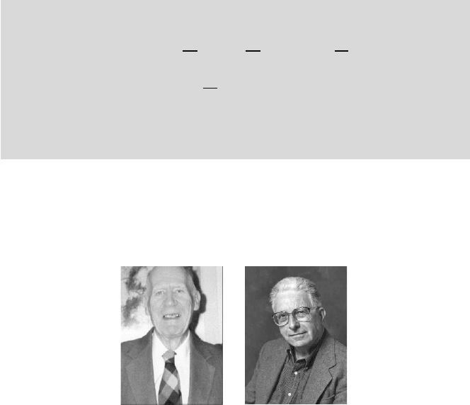
(Fig. 18.1) is the most cited paper in the ﬁeld of statistics (Stigler, 1994).

(a) (b)

Fig. 18.1 (a) Edward Kaplan (1920–2006) and (b) Paul Meier (b. 1924). Kaplan and Meier

never actually met during the time their article was published. They both submitted their

idea for the “product-limit estimator” to the Journal of the American Statistical Association

at approximately the same time, so their results have been merged through mail correspon-

dence.

For uncensored observations, the Kaplan–Meier estimator is identical to

the regular MLE. The difference occurs when there is a censored observation

– then the Kaplan–Meier estimator takes the “weight” normally assigned to

that observation and distributes it evenly among all observed values to the

708 18 Inference for Censored Data and Survival Analysis

right of the observation. This is intuitive because we know that the true value

of the censored observation must be somewhere to the right of the censored

value, but information about what the exact value should be is lacking.

The variance of Kaplan–Meier estimator is estimated by Greenwood’s for-

mula:

Var

S(t)

≤t

−d

)

The pointwise conﬁdence intervals (for a ﬁxed time t

∗

) for the survival

function S(t

∗

) can be found in several ways. The two most popular conﬁdence

intervals are

linear

S(t

∗

) −z

1−α/2

Var

S(t

∗

)

S(t

∗

) +z

1−α/2

Var

S(t

∗

)

and log-transformed

(

S(t

∗

))

1/v

, (

S(t

∗

))

, v =exp











1−α/2

Var

S(t

∗

)

log

S(t

∗

)











Although not centered at

S(t

∗

), the log-transformed interval is considered su-

perior to the linear.

The above pointwise conﬁdence intervals differ from simultaneous conﬁ-

dence bounds on S(t) for which the conﬁdence of 1

−α means that the prob-

ability that any part of the curve S(t) will fall outside the bounds does not

exceed

α. Such general bounds are naturally wider than those generated by

pointwise conﬁdence intervals since the overall conﬁdence is controlled. Two

important types of conﬁdence bands are Nair’s equal precision bands and

the Hall–Wellner bands. These bounds fall beyond the scope of this text; see

Klein and Moeschberger (2003), p. 109, for further discussion and implementa-

tion. The bounds computed in MATLAB’s

[f,t,flo,fup]=ecdf(...) also return

lower and upper conﬁdence bounds for the CDF. These bounds are calculated

by using Greenwood’s formula and are not simultaneous conﬁdence bounds.

The Kaplan–Meier estimator also provides an estimator for the cumulative

hazard H(t) as

18.3 Inference with Censored Observations 709

H(t)

=−log

S(t)

Better small-sample performance in estimating the cumulative hazard

could be achieved by the Nelson–Aalen estimator,

H(t)

, for t > t

H(t) =0, for t ≤ t

with an estimated variance

(t) =

. Using

H(t) and σ

(t), point-

wise conﬁdence intervals on H(t) can be obtained.

Example 18.6. Catheter Complications in Peritoneal Dialysis. The fol-

lowing example is from Chadha et al. (2000). The authors studied a sample

of 36 pediatric patients undergoing acute peritoneal dialysis through Cook

Catheters. They wished to examine how long these catheters performed prop-

erly. They noted the date of complication (either occlusion, leakage, exit-site

infection, or peritonitis).

Half of the subjects had no complications before the catheter was removed.

Reasons for removal of the catheter in this group of patients were that the

patient recovered (n

=4), the patient died (n =9), or the catheter was changed

to a different type electively (n

=5). If the catheter was removed prior to com-

plications, that represented a censored observation, because they knew that

the catheter remained complication free at least until the time of removal.

Day Censored, ` Fail, d At Risk, r 1−(Failures/At Risk) KM

1 8 2 36 1 − 2/36 = 0.944 0.9444

2 2 2 36

− 8 − 2 = 26 1 − 2/26 = 0.92 0.92 · 0.944 = 0.8718

3 1 2 26

− 2 − 2 = 22 1 − 2/22 = 0.91 0.91 · 0.872 = 0.7925

4 1 1 22

− 1 − 2 = 19 1 − 1/19 = 0.95 0.95 · 0.793 = 0.7508

5 6 3 19

− 1 − 1 = 17 1 − 3/17 = 0.82 0.6183

6 0 2 17

− 6 − 3 = 8 1 − 2/8 = 0.75 0.4637

7 0 1 8

− 0 − 2 = 6 1 − 1/6 = 0.83 0.3865

10 0 2 6

− 0 − 1 = 5 1 − 2/5 = 0.60 0.2319

12 0 2 5

− 0 − 2 = 3 1 − 2/3 = 0.33 0.0773

13 0 1 3

− 0 − 2 = 1 1 − 1/1 = 0.00 0.0000

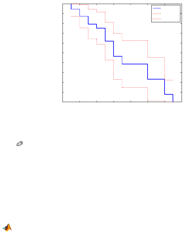
MATLAB script chada.m ﬁnds the Kaplan–Meier estimator and gener-

ates Fig. 18.2. plots

%chada.m

times=[1,1,1,1,1,1,1,1,1,1,2,2,2,2,...

3,3,3,4,4,5,5,5,5,5,5,5,5,5,...

6,6,7,10,10,12,12,13];

censored =[1,1,1,1,1,1,1,1,0,0,1,1,...

0,0,1,0,0,1,0,1,1,1,1,1,...

1,0,0,0,0,0,0,0,0,0,0,0];

% Calculate and plot empirical

% cdf and confidence bounds

[f,x,flo,fup] = ecdf(times,’censoring’,censored);

(1-f)’

710 18 Inference for Censored Data and Survival Analysis

%1.0000 0.9444 0.8718 0.7925 0.7508

%0.6183 0.4637 0.3865 0.2319 0.0773 0

x’

%1 1 2 3 4 5 6 10 12 13

stairs(x,1-f,’LineWidth’,2)

hold on

stairs(x,1-flo,’r:’,’LineWidth’,2)

stairs(x,1-fup,’r:’,’LineWidth’,2)

legend(’Empirical’,’LCB’,’UCB’,...

’Location’,’NE’)

hold off

0 2 4 6 8 10 12 14

0.1

0.2

0.3

0.4

0.5

0.6

0.7

0.8

0.9

Empirical

LCB

UCB

Fig. 18.2 Kaplan–Meier estimator for Catheter Complications data.

Example 18.7. Strength of Weathered Cord. Data from Crowder et al.

(1991) lists strength measurements (in coded units) for 48 pieces of weathered

cord. Seven of the pieces of cord were damaged and yielded strength measure-

ments that are considered right-censored. That is, because the damaged cord

was taken off test, we know only the lower limit of its strength. In the MAT-

LAB code below, the vector

data represents the strength measurements, and

the vector

censor indicates (with a zero) if the corresponding observation in

data is censored.

data=[36.3,41.7,43.9,49.9,50.1,50.8,51.9,52.1,52.3,52.3,...

52.4,52.6,52.7,53.1,53.6,53.6,53.9,53.9,54.1,54.6,...

54.8,54.8,55.1,55.4,55.9,56.0,56.1,56.5,56.9,57.1,...

57.1,57.3,57.7,57.8,58.1,58.9,59.0,59.1,59.6,60.4,...

60.7,26.8,29.6,33.4,35.0,40.0,41.9,42.5];