Troyan V., Kiselev Y. Statistical Methods of Geophysical Data Processing

Подождите немного. Документ загружается.

Ray theory of wave ﬁeld propagation 143

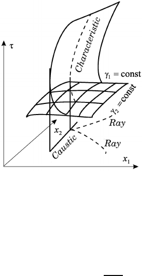
Fig. 5.1 Projection of the characteristic, given in a phase space.

formation of caustics is represented.) For the case of the simplest Hamilton function

H = [(p, p) −n

(x)]/2 this functional reads as

τ =

n(x)dl =

c(x)

with a physical sense as a time of propagation from the point A to the point B.

Here the ray corresponds to the stationary time of propagation. The stationary

condition of the functional τ: δτ = 0 is called Fermat’s principle. The solution of

the appropriate extremum problem forms the basis for the constructing algorithms

of the numerical calculation of rays in inhomogeneous media.

The modern interpretation of the Fermat’s principle bases on the representation

concerning interference of the wave perturbations (Huygens–Kirchhoﬀ principle),

propagating from the point A to the point B on every possible virtual pathways.

Thus, those pathways “survive” only, for which one the variation of the eikonal

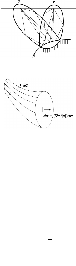
(phase) has a value of ∼ λ/2. In Fig. 5.2 the rays having a common point with

boundary of the Fresnel zone are represented, i.e. taking into account the Fresnel

zone, the contribution of all remaining pathways will be a negligible small quantity

by virtue of a compensation of interfering waves with diﬀerent phases (in calculus

mathematics it corresponds to the stationary phase principle). According to the

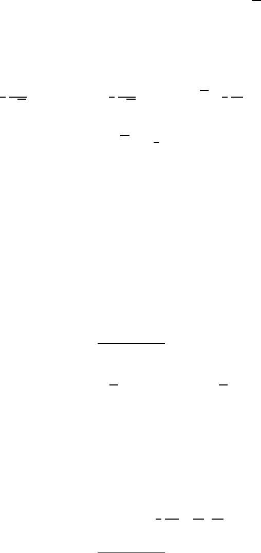
modern interpretation, the the ray concept lies in ray representation by a dimen-

sional ray tube (Fig. 5.3) with a diameter about the ﬁrst Fresnel zone. Let’s mark,

that in a case of the nondispersive medium the Fermat’s principle can be interpreted

as a requirement of a stationarity of the propagation time of a wave from the point

A to the point B.

144 STATISTICAL METHODS OF GEOPHYSICAL DATA PROCESSING

Fig. 5.2 The rays having a common point with boundary of the Fresnel zone.

Fig. 5.3 Space ray tube.

5.3 Shortwave Asymptotic Form of the Solution of the One-

Dimensional Helmholtz Equation (WKB Approximation)

Let us consider one more example of the application of the perturbation theory to

the solution of the Helmholtz equation:

ϕ + V (x)ϕ = 0. (5.21)

In accordance with the perturbation theory we write:

ϕ = exp{iτ(x)}. (5.22)

Then the equation (5.21) has a form

−(τ

)

+ iτ

+ V = 0. (5.23)

Considering τ

being small we obtain τ

= ±

√

V , i.e.

τ(x) = ±

√

V dx. (5.24)

Validity condition of the above approximation is

|τ

| ≈



√



 |V |.

Ray theory of wave ﬁeld propagation 145

With the help of the formulas (5.22) and (5.23) it is to see, that (

√

V )

−1

has a

physical sense of the wavelength (“exponential length”, i.e. it is a character interval

of the variation of V in a case of Imτ > 0). Thus, the approximation (5.24) is valid,

if the variation of V at distance about wavelength is much less, than value of V ,

i.e. V (x) has a small variation in a scale of the wavelength.

Following approximation we shall ﬁnd by solving of the equation (5.23) at

≈ ±

√

, (τ

)

≈ V ±

√

, τ

≈ ±

√

V +

. (5.25)

After integration of the obtained expression and can write down

τ(x) ≈ ±

√

V dx +

ln V. (5.26)

Using approximation (5.26), we can construct a superposition of the solutions

corresponding to the diﬀerent signs. Therefore WKB approximation is valid, if

|∆V (x)| ≤ |V (x)|.

In the sewing point V (x) = 0 is valid, and ∆V (x) is singular, then the exact

solution of the equation (5.21) in this point is a regular solution, while the WKB

solution has singularity in this point. Therefore we ﬁnd the solution ϕ(x) as a speed

key ˜ϕ

and ˜ϕ

−

ϕ(x) = a

˜ϕ

(x) + a

−

˜ϕ

−

(x).

We shall ﬁnd those coeﬃcients using the next equality for ϕ

(x):

(x) = a

˜ϕ

(x) + a

−

˜ϕ

−

(x),

= const, a

−

= const. Solution of this system about a

and a

−

is placed below

ϕ ˜ϕ

−

− ϕ

˜ϕ

−

˜ϕ

−

− ˜ϕ

˜ϕ

−

and for approximation (5.26) we can write

˜ϕ(x) ≈ (V (x))

−1/4



exp



√

V dx



+ c

−

exp



−i

√

V dx



. (5.27)

The solution (5.27) is suitable in any ﬁeld, where the validity condition is satisﬁed,

but it is obviously broken in the vicinity of the point x

: V (x

) = 0, it is necessary

to be able to join of exponential (at V (x) < 0) and oscillating (at V (x) > 0)

solutions, i.e. we need the connecting formulas.

Let’s note, that the WKB solutions (5.27), which we have written in a form ˜ϕ

and ˜ϕ

−

(correspond to c

= 1 and c

−

= 1), are exact solutions for the equation of

(5.21), where V (x) is exchanged by the following expression:

V (x) ⇒ V (x) + ∆V (x)

∆

= V (x) +

−

(

)

−

ϕ ˜ϕ

− ϕ

˜ϕ

−

− ˜ϕ

˜ϕ

−

146 STATISTICAL METHODS OF GEOPHYSICAL DATA PROCESSING

Taking into account that determinant of the system is equal to ˜ϕ

˜ϕ

−

−˜ϕ

˜ϕ

−

= −2i

and ϕ ˜ϕ

∓

− ϕ

˜ϕ

∓

= ∆V (x)ϕ ˜ϕ

∓

, we obtain

= ∓

∆V (x)ϕ ˜ϕ

∓

= ∓

∆V (x)

V (x)







+ a

∓

exp ∓

√

V dx







The above expression is an estimation of the error being able to appear in the WKB

approximation along the large interval ∆x.

5.4 The Elements of Elastic Wave Ray Theory

According to the ray theory of propagation of the seismic wave, body wave prop-

agates with local velocity along the ray (having the jogs on interfaces of elastic

medium, according to a Snell’s law), with the amplitude given by a geometrical

spreading of the ray (Babic and Buldyrev, 1991; Goldin, 1984; Petrashen et al.,

1985). Using the general ray theory (see Sec. 5.1) in the stationary medium, we

represent the eikonal as τ(x, t) as t − τ(x), where τ (x) is called a wavefront. Ap-

plicability of the ray theory is connected with the assumption of much more fast

variation of the wave process in a normal direction to the wavefront (n = ∇

∇

∇τ/|

∇

∇τ|)

in comparison with variations of the characteristics of the medium, i.e. we suppose

a validity of the shortwave asymptotic, when the ratio of the wavelength to the

typical sizes of an inhomogeneity of the medium is a small quantity.

Under the selected eikonal form the wave vector can be represented as p =

; p

, p

) = (p

, p) = (1, ∇∇τ ), where vector p is coaxial to the vector of the

phase velocity (a normal direction to the wavefront) is called a refraction vector.

The Lame operator in the form (4.16) has the vector structure:

L =

Iρ

∂

∂t

− ∇ ·

K∂

here I is an unit operator in R

space. Operator

∂

reads as

∂

a =



∂a

/∂x

∂a

/∂x

∂a

/∂x

∂a

/∂x

∂a

/∂x

∂a

/∂x

∂a

/∂x

∂a

/∂x

∂a

/∂x



Let us write a concrete form of the equation (5.5) for the Lame operator

(ρ

I −

Kp p

= 0. (5.28)

Here (

Kp p

)

ijlk

, p = ∇∇τ. The solvability condition for the

equation (5.28)

det(ρ

I −

Kp p

) = 0 (5.29)

describes the fronts existing in the elastic medium. Let us write down the tensor of

the elastic modules

K for the isotropic elastic medium:

ijkl

= λδ

+ µ(δ

+ δ

Ray theory of wave ﬁeld propagation 147

Choosing a local (ray) orthogonal coordinate frame

|p|

, e

= e

× e

then we write down the coordinate representation of L

(p)A

= 0:



(λ + 2µ)(p · p

) − ρ 0 0

0 µ(p · p

) − ρ 0

0 0 µ(p · p

) − ρ



= 0 . (5.30)

The solvability condition for the system (5.30) leads us to the conclusion that, in

accordance with the ray method, there are three kind of the waves in uniform and

isotropic elastic medium:

(1) quasi-longitudinal wave with the velocity (λ(x) + 2µ(x))/ρ(x)

∆

= c

(x) and the

polarization vector coinciding with e

, which describes by the eikonal equation:

(p · p) =

ρ(x)

λ(x) + 2µ(x)

;

(2) quasi-shear waves of two kinds with polarisation vectors e

and e

, propagat-

ing with equal velocities µ(x)/ρ(x)

∆

= c

(x), which are describes by equation

(p · p) = ρ(x)/µ(x).

5.5 The Ray Description of Almost-Stratiﬁed Medium

The propagation of an acoustic wave at ocean is well approximated by the model

of the almost-stratiﬁed medium, i.e. the medium with smoothly varying (in com-

parison with depth) velocity of the wave propagation in a horizontal direction.

Following the logic of Sec. 5.1, we shall consider horizontal coordinates ρ = (x, y) as

“slow” arguments, and vertical coordinate z — as a “fast” argument, i.e. velocity

c = c(αx, αy, z).

The wave equation for the time component of the Fourier transform, in the

spatial domain that does not contain the sources (4.41), reduces to the Helmholtz

equation:



∂

∂x

∂

∂y

∂

∂z

+ k

(αx, αy, z)



ϕ = 0, (5.31)

Let’s in the spatial domain in which the solution of the above equation is consid-

ered for the interfaces of the water column Z

= Z

(αx, αy) the next boundary

condition is valid

(αx, αy)I ±b

(αx, αy)(n · ∇)]



ϕ = 0, (5.32)

148 STATISTICAL METHODS OF GEOPHYSICAL DATA PROCESSING

where a

, b

are the real quantities and



1 +



∂Z

∂x





∂Z

∂y



−1/2



−

∂Z

∂x

, −

∂Z

∂y

, 1



is an outer normal vector. Let us write (5.31) and boundary conditions (5.32) in

the form Lϕ = 0:

L =



where operator

Γ in an explicit form allows the argument of the asymptotic expan-

sion.

Compressing the horizontal coordinates, we make the variation scale of the ve-

locity be the same in the all directions x

= αx, y

= αy, z

= z. In the new

coordinates the operator L looks like

L =>





∂

∂x

∂

∂y





∂

∂z

+ k

, y

, z

)



∆

= α

∆

, (5.33)

Γ =>



I + b



∂

∂z

− α

· ∇

)





. (5.34)

Taking into account the asymptotic representation

ϕ ∼ A(x

, y

, z

; α) exp



τ(x

, y

)



the solvability condition (5.5) (with the presence of the boundary conditions (5.34))

can be written as

−i(∇

τ·ρ)

∆

i(∇

τ·ρ)

= 0,

∆



I + b

∂

∂z



= 0,

where

ρ = (x, y), i.e.

[(∇∇τ ·∇∇τ) −

= 0, (5.35)



= 0. (5.36)

The equation (5.35) leads to the problem of eigenvalues and eigenfunctions of the

operator

with boundary conditions (5.36):

= λ



= 0, (5.37)

where

= (∇∇τ ·∇∇τ). (5.38)

Ray theory of wave ﬁeld propagation 149

Let us consider the equation (5.37) (omitting the zero index):

∂

∂z



x,y

(z)

− λ



= 0,



x,y

+ b

∂

∂z



x,y

= 0.

Introducing the notations c

x,y

(z), Z

x,y

, we underscore “slow” arguments, i.e. we

consider the eigenfunction and eigenvalue problem (Sturm–Liouville problem) as

parametric one, which depends on a point (x, y).

Equation (5.37) can be solved by WKB method (see. Sec. 5.3), which allows us

to ﬁnd the short-wave asymptotic for amplitude A

. It is obviously that eigenvalues

depend on the interface position Z

x,y

, the frequency ω and the depth dependence

of the velocity:

= λ

x,y

, ω, c

x,y

(z)).

It is possible to solve the equation (5.38) (eikonal equation) by the method of

characteristics (see Sec. 5.2):

dρρ

= p,

∇∇λ

(ρ),

dτ

= (p · p),

dτ

= λ

(ρ).

Let us represent the amplitude A

in the form

= A

(x, y, z) = a

(x, y)ψ

(x, y, z),

where {ψ

} is an orthonormal basis of the operator,

−

dz = δ

. Therefore

it is possible to obtain the transport equation for reduced amplitude a

, which

depends on horizontal coordinate only; in accordance with formula (5.6) we can

write:

∇

τ + 2(

∇

∇τ ·

∇

∇a

) = 0.

It is possible to represent the transport equation as:

∇∇ · (a

∇τ) = 0. (5.39)

Integrating (5.39) on the ray tube volume (see Fig. 5.3)and using the Gauss theorem,

we obtain

·∇

∇

∇τ) · dσ

σ = 0.

Taking into account that the tube cross-section is represented as d

σ = ∇∇τ/|∇τ|σ,

and at the tube wall is valid ∇τ ·dσ = 0, we can write: λ

·∆σ = const. Here ∆σ

is a square of the tube cross-section, i.e. reduced amplitude varies as a

∼ r

−1/2

For space-time ray, using asymptotic representation

ϕ ∼ A(x

, y

, z, t

; α) exp



τ(x

, y

, t

)



150 STATISTICAL METHODS OF GEOPHYSICAL DATA PROCESSING

we obtain

= λ

(ω, x, y, [c(z)], t)

and, respectively, the eikonal equation reads as

(∇τ · ∇τ ) = λ

(ω, x, y, [c(z)], t). (5.40)

Taking into consideration (5.40), the characteristic equations can be represented as

∂

dτ

(λ

− ω∂

)

∂

= −

dω

∂

(5.41)

= ∂/∂x τ, p

= ∂/∂y τ)

and deﬁne the horizontal space-time rays.

After diﬀerentiation of (5.40) on p = (p

, p

) and taking into consideration that

ω = ω(p), we obtain

p = λ

∂

∇

ω. (5.42)

Using the ﬁrst two equalities from (5.41) and equation (5.42), we can write

dρρ

∂

= ∇

ω.

Hence, the horizontal space-time rays determine the trajectories of points that

move with the group velocity.

Let us consider representation of the exact solution of the problem (5.31), (5.32)

in a form of the normal modes for a stratiﬁed ocean. Each normal mode is a solution

of the equation (5.31) with separated variables:

ϕ(z, ρ) = ϕ

(z)ϕ

(ρ),



∂

∂z

+ (k

(z) − λ

)



(z) = 0, (5.43)



ϕ(z) = 0,



∂

∂ρ



∂

∂ρ



+ λ



(ρ) = 0,



∞

= 0. (5.44)

At Fig. 5.4 the system of rays into the sound channel with bounds z

, z

, which are

turning points (in terms of WKB method), is represented.

The Sturm–Liouville problem (5.43) has an inﬁnite number of simple real eigen-

values λ

> λ

> > . . ., where λ

: λ

> 0 is the ﬁnite number and λ

< 0

is the inﬁnite number. We should choose λ

> 0, if λ

> 0, and Imλ

> 0, if

Ray theory of wave ﬁeld propagation 151

Fig. 5.4 The system of rays in the sound channel.

< 0. In this case the solution of the equation (5.44) ϕ

satisﬁes under λ = λ

the radiation condition:

lim

ρ−→∞

1/2



∂

∂ρ

− iλϕ



= 0

and it is proportional to the Hankel function H

(1)

(λ

ρ):

∼ H

(1)

(λ

ρ).

Thus, the exact solution ϕ(z, ρ) of the homogeneous equation (5.31) with the

use of the basis {ϕ

(z)} of the equations (5.43) can be represented as inﬁnite series:

ϕ(z, ρ) =

∞

n=0

−

(1)

(λ

ρ). (5.45)

Using the above expression, let us to write the solution of the wave equation with

the point source

(∇

+ k

)ϕ = −δ(z − z

)

δ(ρ)

2πρ

. (5.46)

For this purpose we shall take the advantage of the equality



∂

∂ρ



∂

∂ρ



+ λ



(1)

(λ

ρ) =

4iδ(ρ)

2πρ

Substituting the solution (5.45) of the homogeneous equation (5.31) to the ex-

pression (5.46), we obtain the connection of the coeﬃcients A

and eigenfunctions

(z):

∞

n=0

δ(z − z

Hence, making the scalar product of the above equality with ϕ

, we obtain

The exact solution of the acoustic equation describing propagation of the signal,

generated by the point source at the depth z

, has the next representation in a

stratiﬁed ocean with a constant depth

ϕ(ρ, z) =

∞

n=0

)ϕ

(z)H

(1)

(λ

ρ). (5.47)

152 STATISTICAL METHODS OF GEOPHYSICAL DATA PROCESSING

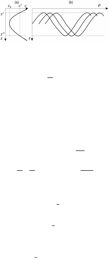
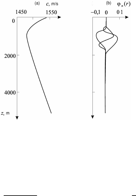
Fig. 5.5 The typical proﬁle of the sound velocity in ocean (a) and the ﬁrst tree modes (b).

At Fig. 5.5 a typical sound velocity proﬁle in ocean (a) and the ﬁrst three modes

for the frequency 30 Hz (b) are represented.

The asymptotic of the exact solution (5.47) in the wave zone (ρ is great enough),

using asymptotic for the Hankel function, can be written as

ϕ(ρ, z)

ρ→∞

∼

3/2

1/2

∞

n=0

1/2

)ϕ

(z) exp





ρ −



. (5.48)

(We will use the expressions (5.48) for the development of the algorithms.)

5.6 Surface Wave in Vertically Inhomogeneous Medium

At study of a crystal structure and the upper earth mantle, the information con-

tained in the surface waves which extracted on the seismograms is widely used,

because their signal-to-noise merit has enough high magnitude in comparison with

the body waves (an amplitude of surface waves are described by the factor r

−1/2

and

for the body waves this factor is r

−1

). Transiting through an area with a various

geological feature, the waves accumulate the information on elastic properties and

a geometry of these areas. This information is most concentrated in dependence

of the velocity of propagation on frequency. In turn, the extraction of the surface

waves is guaranteed by a presence of the polarization.

At a long-range propagation of the ground waves allows the ray method and to

take advantage of the asymptotic expansion similar to the expansion of the acoustic