Trauth M.H., MATLAB® Recipes for Earth Sciences, Third edition

Подождите немного. Документ загружается.

298 9 MULTIVARIATE STATISTICS

load of B1. Again, the high in uence of B2 with an opposite sign re ects the

weathering of B1 to produce B2.  e occurrence of B3 in both source rocks

results in high loads of B3 in both PC

and PC

. Principle components PC

and PC

show mixed and contradictory patterns of loads and are therefore

not easy to interpret, most probably as a result of noise in the data set.

An alternative way to plot of the loads is as a bivariate plot of two princi-

pal components. We therefore ignore PC

and PC

at this point and concen-

trate on PC

and PC

. Remember to either close the  gure window before

plotting the loads or clear the  gure window using

clf, in order to avoid

integrating the new plot as a fourth subplot in the previous  gure window.

plot(pcs(:,1),pcs(:,2),'o'), hold on

text(pcs(:,1)+0.02,pcs(:,2),minerals,'FontSize',14)

plot([-0.8 0.8],[0 0],'r')

plot([0 0],[-0.8 0.8],'r')

xlabel('First Principal Component Loads')

ylabel('Second Principal Component Loads')

hold off

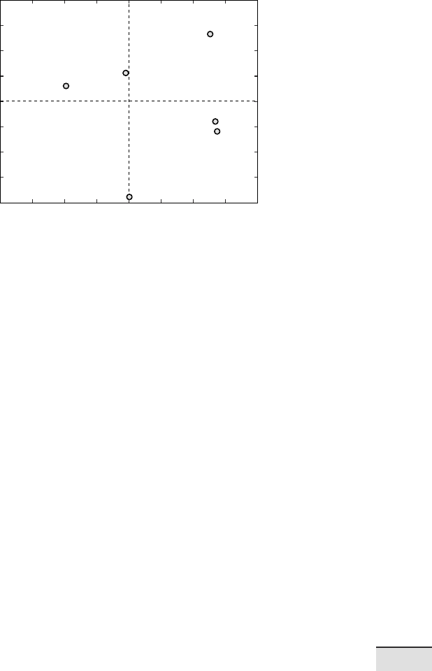
We can now observe in a single plot the same relationships that were previ-

ously shown on several graphs (Fig. 9.3). It is also possible to plot the data

set as functions of the new variables.  is requires the second output of

princomp, containing the principal component scores.

plot(newdata(:,1),newdata(:,2),'+'), hold on

text(newdata(:,1)+0.01,newdata(:,2),sample)

plot([-80 100],[0 0],'r')

plot([0 0],[-60 80],'r')

xlabel('First Principal Component Scores')

ylabel('Second Principal Component Scores')

hold off

 is plot clearly de nes groups of samples with similar in uences. Samples

5, 8, 20, 27 and 30, dominated by in uences of the  rst source rock, all clus-

ter in the right half of the diagram, while samples 7, 9, 24 and once again 30,

strongly in uenced by the second rock type, all fall in the upper half of the

graph. Next, we use the third output of the function

princomp to compute

the variances of the PCs.

percent_explained = 100*variances/sum(variances)

percent_explained =

72.7390

14.6658

4.3129

4.1775

2.7791

1.3257

9.2 PRINCIPAL COMPONENT ANALYSIS 299

9 MULTIVARIATE STATISTICS

MinA1

MinA2

MinA3

MinB1

MinB2

MinB3

−0.6 −0.4

−0.2

0.2 0.4 0.6 0.8

−0.8

−0.6

−0.4

−0.2

0.4

0.2

0.6

0.8

First Principal Component Loads

Second Principal Component Loads

Fig. 9.3 Principal components suggesting that the PCs are in uenced by di erent minerals.

See text for detailed interpretation of the PCs.

We see that almost 73 % of the total variance is contained in PC

, and around

15 % is contained in PC

, while none of the other PCs contribute very much

to the total variance of the data set.  is means that most of the variability

in the data set can be described by just two new variables. As would be ex-

pected, the two new variables do not correlate with each other as illustrated

by a correlation coe cient between

newdata(:,1) and newdata(:,2)

that is close to zero.

corrcoef(newdata(:,1),newdata(:,2))

ans =

1.0000 0.0000

0.0000 1.0000

We can therefore plot the time series of the thirty samples as two indepen-

dent variables PC

and PC

, in a single plot.

plot(1:30,newdata(:,1),1:30,newdata(:,2)), grid,

legend('PC1','PC2')

xlabel('Sample ID'), ylabel('Value')

 is plot displays ca. 73 %+15 %=88 % of the variance contained in the mul-

tivariate data set. According to our interpretation of PC

and PC

this plot

shows the variability in the relative contributions from the two sources to

the sedimentary column under investigation.

In summary, the approach described above has been used to study the

300 9 MULTIVARIATE STATISTICS

provenance of varved lake sediments deposited around 33 kyrs ago in a

landslide-dammed lake in the Quebrada de Cafayate (Trauth et al. 2003).

 e provenance of the sediments contained in the varved layers can be

traced using index minerals characteristic of the various possible watershed

source areas. A comparison of the mineral assemblages in the sediments

with those of potential source rocks within the catchment area indicates

that Fe-rich Tertiary sedimentary rocks exposed in the Santa Maria Basin

were the source of the red-colored basal portion of the varves. In contrast,

metamorphic rocks in the mountainous parts of the catchment area were

the most likely source of the relatively drab-colored upper part of the varves

(see also Section 8.7).

9.3 Independent Component Analysis (by N. Marwan)

Principal component analysis (PCA) is the standard method for separating

mixed signals. Such analyses produce signals that are linearly uncorrelated.

 is method is also called whitening since this property is characteristic of

white noise. Although the separated signals are uncorrelated, they can still

be interdependent, i.e., nonlinear correlation may still remain.  e inde-

pendent component analysis (ICA) was developed to investigate such data.

It separates mixed signals into independent signals, which are then non-

linearly uncorrelated. Fast ICA algorithms use a criterion that estimates

how Gaussian the combined distribution of the independent components is.

 e less Gaussian this distribution is, the more independent the individual

components are.

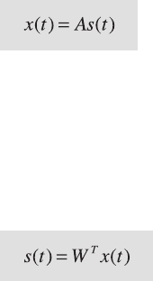
According to the model, n independent signals x(t) are linearly mixed

in m measurements,

in which we are interested in the source signals s

and the mixing matrix A.

For example, we can imagine that we are at a party in which a lot of people

are carrying on independent conversations. We can hear a mixture of these

conversations but perhaps cannot distinguish them individually. We could

install some microphones and use these to separate out the individual con-

versations: hence, this dilemma is sometimes known as the cocktail party

problem. Its correct term is blind source separation, which is de ned by

9.3 INDEPENDENT COMPONENT ANALYSIS (BY N. MARWAN) 301

9 MULTIVARIATE STATISTICS

where W

is the separation matrix required to reverse the mixing and ob-

tain the original signals. Let us consider a mixing of three signals, s

, s

and

, and their separation using PCA and ICA. First, we create three periodic

signals

clear

i = (1:0.01:10 * pi)';

[dummy index] = sort(sin(i));

s1(index,1) = i/31; s1 = s1 - mean(s1);

s2 = abs(cos(1.89*i)); s2 = s2 - mean(s2);

s3 = sin(3.43*i);

subplot(3,2,1), plot(s1), ylabel('s_1'), title('Raw signals')

subplot(3,2,3), plot(s2), ylabel('s_2')

subplot(3,2,5), plot(s3), ylabel('s_3')

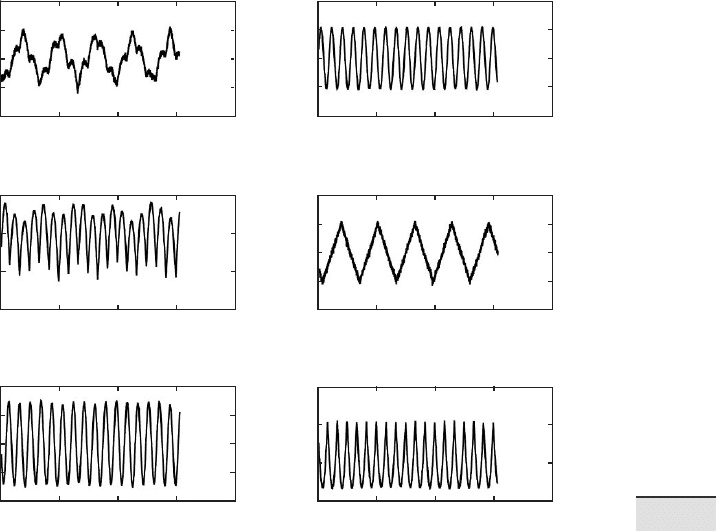
Now we mix these signals and add some observational noise. We obtain a

three-column vector

x which corresponds to our measurements (Fig. 9.4).

randn('state',1);

x = [.1*s1 + .8*s2 + .01*randn(length(i),1), ...

.4*s1 + .3*s2 + .01*randn(length(i),1), ...

.1*s1 + s3 + .02*randn(length(i),1)];

subplot(3,2,2), plot(x(:,1)), ylabel('x_1'), title('Mixed

signals')

subplot(3,2,4), plot(x(:,2)), ylabel('x_2')

subplot(3,2,6), plot(x(:,3)), ylabel('x_3')

We begin with the separation of the signals using PCA. We calculate the

principal components and the whitening matrix

W_PCA with

[E sPCA D] = princomp(x);

sPCA = sPCA./repmat(std(sPCA),length(sPCA),1);

 e PC scores sPCA are the linearly separated components of the mixed

signals x (Fig. 9.5).

subplot(3,2,1), plot(sPCA(:,1))

ylabel('s_{PCA1}'), title('Separated signals - PCA')

subplot(3,2,3), plot(sPCA(:,2)), ylabel('s_{PCA2}')

subplot(3,2,5), plot(sPCA(:,3)), ylabel('s_{PCA3}')

 e mixing matrix A can be found with

A_PCA = E * sqrt(diag(D));

W_PCA = inv(sqrt(diag(D))) * E';

302 9 MULTIVARIATE STATISTICS

0 1000 2000 3000 4000

1000

2000

3000

4000

0 1000 2000 3000 4000

−2

−1

−0.4

−0.2

0.2

0.4

−1.0

−0.5

0.5

−1.0

−0.5

0.5

1.0

−1.0

−0.5

0.5

−0.5

0.5

Raw Signals Mixed Signals

e f

Fig. 9.4 Sample input for the independent component analysis. We  rst generate three

period signals (a, c, e), mix the signals and add some Gausssian noise (b, d, f).

Next, we separate the signals into independent components. We will do

this by using a FastICA algorithm, which is based on a  xed-point iteration

scheme, to  nd the least Gaussian distributed of the independent compo-

nents W

x. For the nonlinearity function we use a power of three function,

as an example,

rand('state',1);

div = 0;

B = orth(rand(3, 3) - .5);

BOld = zeros(size(B));

while (1 - div) > eps

B = B * real(inv(B' * B)^(1/2));

div = min(abs(diag(B' * BOld)));

BOld = B;

9.3 INDEPENDENT COMPONENT ANALYSIS (BY N. MARWAN) 303

9 MULTIVARIATE STATISTICS

0 1000 2000 3000 4000

1000

2000

3000

4000

0 1000 2000 3000 4000

−4

−2

−4

−2

−1

−4

−2

−4

−2

sss

PCA1PCA2PCA3

ICA1

ICA2

ICA3

Separated Signals − PCA

Separated Signals − ICA

e f

Fig. 9.5 Output of the principal component analysis (a, c, e) compared with the output of

the independent component analysis (b, d, f).  e PCA has not reliably separated the mixed

signals, whereas the ICA identi ed the source signals almost perfectly.

B = (sPCA' * (sPCA * B) .^ 3) / length(sPCA) - 3 * B;

sICA = sPCA * B;

end

We plot the separated components (Fig. 9.5) with

subplot(3,2,2), plot(sICA(:,1)), ylabel('s_{ICA1}'),

title('Separated signals - ICA')

subplot(3,2,4), plot(sICA(:,2)), ylabel('s_{ICA2}')

subplot(3,2,6), plot(sICA(:,3)), ylabel('s_{ICA3}')

We can now see that the PCA algorithm has not provided a satisfactory

separation of the mixed signals.  e saw-tooth signal, in particular, was not

correctly identi ed. In contrast, the ICA has identi ed the source signals

almost perfectly.  e only noticeable di erences are the noise level, which

304 9 MULTIVARIATE STATISTICS

derives from the observations, the incorrect sign, and the incorrect order

of the signals. However, the sign and the order of the signals are not really

important, since we generally do not have any knowledge of the real sources

or of their order. With

A_ICA = A_PCA * B;

W_ICA = B' * W_PCA;

we compute the mixing matrix A and the separation matrix W.  e mixing

matrix A can be used to estimate the proportions of the separated signals in

our measurements  e components a

of the mixing matrix A correspond

to the principal component loads, as introduced in Section 9.2. A FastICA

package is available for MATLAB and can be found at

http://www.cis.hut.fi/projects/ica/fastica/

9.4 Cluster Analysis

Cluster analysis creates groups of objects that are very similar to each other,

compared to other individual objects or groups of objects. It  rst computes

the similarity between all pairs of objects, and then ranks the groups ac-

cording to their similarity,  nally creating a hierarchical tree visualized as

a dendrogram. Examples for grouping objects in earth sciences are correla-

tions within volcanic ash layers (Hermanns et al. 2000) and comparisons

between microfossil assemblages (Birks and Gordon 1985).

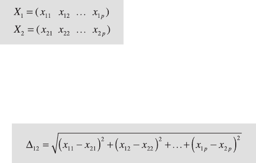
 ere are numerous methods for calculating the similarity between two

data vectors. Let us de ne two data sets consisting of multiple measure-

ments on the same object.  ese data can be described by vectors.

 e most popular measures of similarity between the two sample vectors

are the

Euclidian distance• –  is is simply the shortest distance between the two

points describing two measurements in the multivariate space:

9.4 CLUSTER ANALYSIS 305

9 MULTIVARIATE STATISTICS

 e Euclidian distance is certainly the most intuitive measure for simi-

larity. However, in heterogeneous data sets consisting of a number of dif-

ferent types of variables, a better alternative would be the

• Manhattan distance – In the city of Manhattan, one must walk along

perpendicular avenues rather than crossing blocks diagonally.  e

Manhattan distance is therefore the sum of all di erences:

Other alternative measures of similarity include the

• Correlation similarity coefficient –  is uses Pearson’s linear product-

moment correlation coe cient to compute the similarity of two objects:

 is measure is used if one is interested in the ratios between the vari-

ables measured on the objects. However, Pearson’s correlation coe -

cient is highly sensitive to outliers and should be used with care (see also

Section 4.2).

• Inner-product similarity index – Normalizing the length of the data vec-

tors to a value of one and computing the inner product of these yields

another important similarity index that is o en used in transfer function

applications. In this example, a set of modern  ora or fauna assemblages

with known environmental preferences is compared with a fossil sample

to reconstruct the environmental conditions in the past.

 e inner-product similarity varies between 0 and 1. A zero value sug-

gests no similarity and a value of one represents maximum similarity.

306 9 MULTIVARIATE STATISTICS

 e second step in performing a cluster analysis is to rank the groups by

their similarity and build a hierarchical tree visualized as a dendrogram.

Most clustering algorithms simply link the two objects with the highest

level of similarity. In the following steps, the most similar pairs of objects or

clusters are linked iteratively.  e di erence between clusters, each made up

of groups of objects, is described in di erent ways depending on the type of

data and the application.

• K-means clustering – Here, the Euclidean distance between the multi-

variate means of a number of K clusters is used as a measure of the dif-

ference between the groups of objects.  is distance is used if the data

suggest that there is a true mean value surrounded by random noise.

• K-nearest-neighbors clustering – Alternatively, the Euclidean distance of

the nearest neighbors is used as measure of this di erence.  is is used

if there is a natural heterogeneity in the data set that is not attributed to

random noise.

It is important to evaluate the data properties prior to the application of

a clustering algorithm.  e absolute values of the variables should  rst be

considered. For example, a geochemical sample from volcanic ash might

show an SiO

content of around 77 % and a Na

O contents of only 3.5 %, but

the Na

O content may be considered to be of greater importance. Here, the

data need to be transformed to zero means ( mean centering). Di erences

in both the variances and the means are corrected by autoscaling, i.e., the

data are standardized to zero means and variances equal to one. Artifacts

arising from closed data, such as arti cial negative correlations, are avoided

by using Aitchison’s log-ratio transformation (Aitchison 1984, 1986).  is

ensures data independence and avoids the constant sum normalization

constraints.  e log-ratio transformation is

where x

denotes the transformed score (i=1, 2, 3, …, d–1) of some raw data

.  e procedure is invariant under the group of permutations of the vari-

ables, and any variable can be used as the divisor x

As an example for performing a cluster analysis, the sediment data

stored in sediment_2.txt are loaded.  is data set contains the percent-

ages of various minerals contained in sediment samples.  e sediments

are sourced from three rock types: a magmatic rock containing amphibole

9.4 CLUSTER ANALYSIS 307

9 MULTIVARIATE STATISTICS

(amp), pyroxene (pyr) and plagioclase (pla), a hydrothermal vein character-

ized by the occurrence of  uorite (flu), sphalerite (sph) and galena (gal), as

well as some feldspars (plagioclase and potassium feldspars, ksp) and quartz,

and a sandstone unit containing feldspars, quartz and clay minerals (cla).

Ten samples were taken from various levels in this sedimentary sequence

containing varying amounts of these minerals. First, the distances between

pairs of samples can be computed.  e function

pdist provides many ways

for computing this distance, such as the Euclidian or Manhattan city block

distance. We use the default setting which is the Euclidian distance.

clear

data = load('sediments_2.txt');

Y = pdist(data);

 e function pdist returns a vector Y containing the distances between

each pair of observations in the original data matrix. We can visualize the

distances in another pseudocolor plot.

imagesc( squareform(Y)), colormap(hot)

title('Euclidean distance between pairs of samples')

xlabel('First Sample No.')

ylabel('Second Sample No.')

colorbar

 e function squareform converts Y into a symmetric, square format,

so that the elements

(i,j) of the matrix denote the distance between the

i and j objects in the original data. Next, we rank and link the samples

with respect to the inverse of their separation distances using the function

linkage.

Z = linkage(Y)

Z =

2.0000 9.0000 0.0564

8.0000 10.0000 0.0730

1.0000 12.0000 0.0923

6.0000 7.0000 0.1022

11.0000 13.0000 0.1129

3.0000 4.0000 0.1604

15.0000 16.0000 0.1737

5.0000 17.0000 0.1764

14.0000 18.0000 0.2146

In this 3-column array Z, each row identi es a link.  e  rst two columns

identify the objects (or samples) that have been linked, while the third col-

umn contains the separation distance between these two objects.  e  rst