Trauth M.H., MATLAB® Recipes for Earth Sciences, Third edition
Подождите немного. Документ загружается.

238 7 SPATIAL DATA
rithmic transformation if the skewness exceeds 1. A general transformation
formula is:
for min(z)+m>0. is is the so called Box-Cox transform with the special
case k=0 when a logarithm transformation is used. In the logarithm trans-
formation, m should be added if z is zero or negative. Interpolation results
of power-transformed values can be back-transformed directly a er kriging.
e back-transformation of log-transformed values is slightly more com-
plicated and will be explained later. e procedure is known as lognormal
kriging. It can be important because lognormal distributions are not un-
common in geology.
Variography with the Classical Variogram
A variogram describes the spatial dependency of referenced observations
in a uni- or multidimensional space. Since the true variogram of the spatial
process is usually unkown, it has to be estimated from observations. is
procedure is called variography. Variography starts by calculating the ex-
perimental variogram from the raw data. In the next step, the experimen-
tal variogram is summarized by the variogram estimator. e variography
then concludes by tting a variogram model to the variogram estimator.
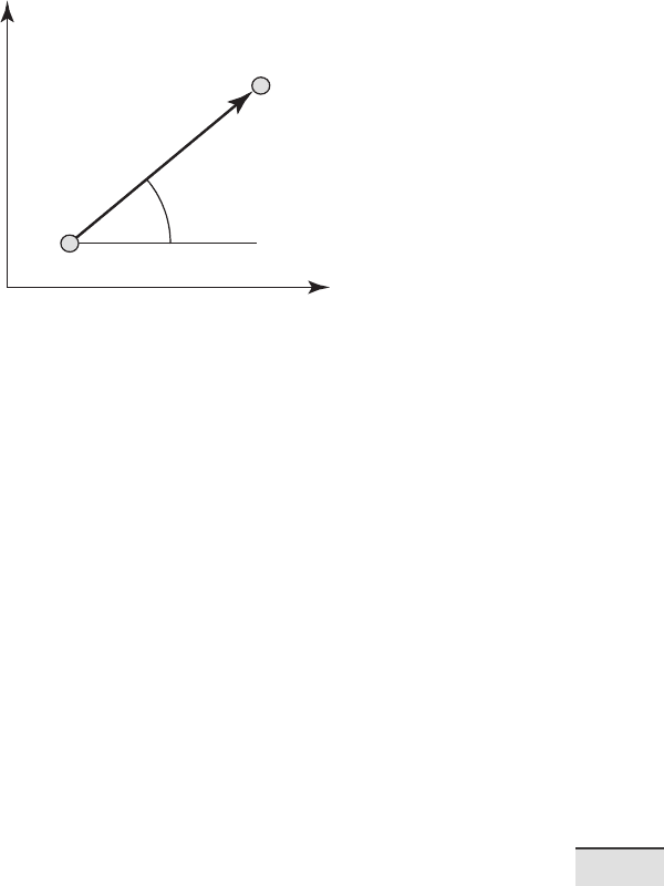
e experimental variogram is calculated as the di erences between pairs of
the observed values, and is dependent on the separation vector h (Fig. 7.17).
e classical experimental variogram is de ned by the semivariance,
where z
x
is the observed value at location x and z
x+h
is the observed value at
another point at a distance h. e length of the separation vector h is called
the lag distance or simply the lag. e correct term for γ(h) is the semivar-
iogram (or semivariance), where semi refers to the fact that it is half of the
variance of the di erence between z
x
and z
x+h
. It is, nevertheless, the vari-
ance per point when points are considered as in pairs (Webster and Oliver,
2001). Conventionally, γ(h) is termed variogram instead of semivariogram,
a convention that we shall follow for the rest of this section. To calculate the
experimental variogram we rst need to group pairs of observations. is
7.11 GEOSTATISTICS AND KRIGING (BY R. GEBBERS) 239
7 SPATIAL DATA
y-Coordinates
x-Coordinates
α
|h|
x = x + h
ji
x
i
Fig. 7.17 Separation vector h between two points.
is achieved by typing
[X1,X2] = meshgrid(x);
[Y1,Y2] = meshgrid(y);
[Z1,Z2] = meshgrid(z);
e matrix of separation distances D between the observation points is
D = sqrt((X1 - X2).^2 + (Y1 - Y2).^2);
We then get the experimental variogram G as half the squared di erences
between the observed values:
G = 0.5*(Z1 - Z2).^2;
In order to to speed up the processing we use the MATLAB capability to
vectorize commands instead of using for loops to run faster. However, we
have computed n
2
pairs of observations although only n(n–1)/2 pairs are
required. For large data sets, e. g., more than 3,000 data points, the so -
ware and physical memory of the computer may become limiting factors. In
such cases, a more e cient method of programming is described in the user
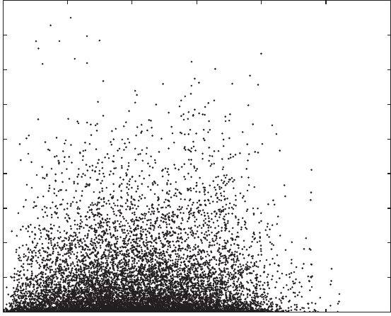
manual for the SURFER so ware (SURFER 2002). e plot of the experi-
mental variogram is called the variogram cloud (Fig. 7.18), which we obtain
by extracting the lower triangular portions of the
D and G arrays.
indx = 1:length(z);
[C,R] = meshgrid(indx);
I = R > C;
240 7 SPATIAL DATA
Distance between observations
Semivariance
0
1
2
3
4
5
6
7
8
9
0 50 100 150 200 250 300
Fig. 7.18 Variogram cloud: Plot of the experimental variogram (half the squared di erence
between pairs of observations) versus the lag distance (separation distance between the two
components of a pair).
plot(D(I),G(I),'.' )
xlabel('lag distance')
ylabel('variogram')
e variogram cloud provides a visual impression of the dispersion of val-
ues at the di erent lags. It can be useful for detecting outliers or anomalies,
but it is hard to judge from this presentation whether there is any spatial
correlation, and if so, what form it might have and how we could model it
(Webster and Oliver 2001). To obtain a clearer view and to prepare a vario-
gram model the experimental variogram is now replaced by the variogram
estimator.
e variogram estimator is derived from the experimental variograms
in order to summarize their central tendency (similar to the descriptive
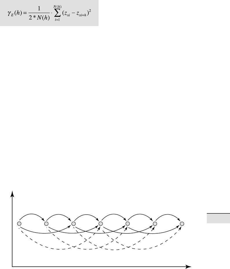
statistics derived from univariate observations, Section 3.2). e classical
variogram estimator is the averaged empirical variogram within certain
distance classes or bins de ned by multiples of the lag interval. e clas-
si cation of separation distances is illustrated in Figure 7.19.
7.11 GEOSTATISTICS AND KRIGING (BY R. GEBBERS) 241
7 SPATIAL DATA
h
3
h
3
h
3
h
3
h
1
h
1
h
1
h
1
h
1
h
1
h
2
h
2
h
2
h
2
h
2
y-Coordinates
x-Coordinates
Fig. 7.19 Classi cation of separation distances for observations that are equally spaced.
e lag interval is h
1
, and h
2
, h
3
etc. are multiples of the lag interval.
e variogram estimator is calculated by:
where N(h) is the number of pairs within the lag interval h.
We rst need to decide on a suitable lag interval h. If sampling has been
carried out on a regular grid, the length of a grid cell can be used. If the
samples are unevenly spaced, as in our case, the mean minimum distance
of pairs is a good starting point for the lag interval (Webster and Oliver
2001). To calculate the mean minimum distance of pairs we need to replace
the zeros in the diagonal of the lag matrix
D with NaNs, otherwise the mean
minimum distance will be zero:
D2 = D.*(diag(x*NaN)+1);
lag = mean(min(D2))
lag =
8.0107
Since the estimated variogram values tend to become more erratic with in-
creasing distances, it is important to place a maximum distance limit on the
calculation. As a rule of thumb, half of the maximum distance is a suitable
limit for variogram analysis. We obtain the half maximum distance and the
maximum number of lags by:
242 7 SPATIAL DATA
hmd = max(D(:))/2
hmd =
130.1901
max_lags = floor(hmd/lag)
max_lags =
16
e separation distances are then classi ed and the classical variogram es-
timator is calculated:
LAGS = ceil(D/lag);
for i = 1 : max_lags
SEL = (LAGS == i);
DE(i) = mean(mean(D(SEL)));
PN(i) = sum(sum(SEL == 1))/2;
GE(i) = mean(mean(G(SEL)));
end
where SEL is the selection matrix de ned by the lag classes in LAG, DE is
the mean lag,
PN is the number of pairs and GE is the variogram estimator.
We can now plot the classical variogram estimator (variogram versus mean
separation distance) together with the population variance:
plot(DE,GE,'.' )
var_z = var(z);
b = [0 max(DE)];
c = [var_z var_z];
hold on
plot(b,c, '--r')
yl = 1.1 * max(GE);
ylim([0 yl])
xlabel('Averaged distance between observations')
ylabel('Averaged semivariance')
hold off
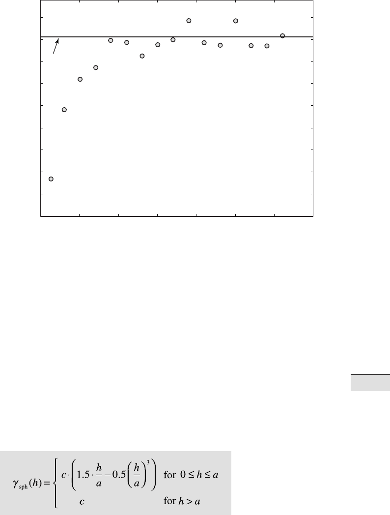
e variogram in Figure 7.20 exhibits a typical pattern of behavior. Values
are low at small separation distances (near the origin), they increase with
increasing distances until reaching a plateau ( sill) which is close to the pop-
ulation variance. is indicates that the spatial process is correlated over
short distances while there is no spatial dependency over longer distances.
e extent of the spatial dependency is called the range and is de ned as the
separation distance at which the variogram reaches the sill.
e variogram model is a parametric curve tted to the variogram es-
timator. is is similar to frequency distribution tting (see Section 3.5),
7.11 GEOSTATISTICS AND KRIGING (BY R. GEBBERS) 243
7 SPATIAL DATA
Population
variance
Distance between observations
Semivariance
0 20 40 60 80 100 120 140
0.1
0.2
0.3
0.4
0.5
0.6
0.7
0.8
0.9
0
Fig. 7.20 e classical variogram estimator (dots) and the population variance (dashed
line).
where the frequency distribution is modeled by a distribution type and its
parameters (e. g., a normal distribution with its mean and variance). For
theoretical reasons, only functions with certain properties should be used
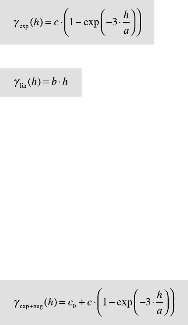
as variogram models. Common authorized models are the spherical, the
exponential and the linear model (more models can be found in the litera-
ture).
Spherical model:
244 7 SPATIAL DATA
Exponential model:
Linear model:
where c is the sill, a is the range, and b is the slope (for a linear model). e
parameters c and either a or b must be modi ed if a variogram model is t-
ted to the variogram estimator. e so called nugget effect is a special type
of variogram model. In practice, when extrapolating the variogram towards
a separation distance of zero, we o en observe a positive intercept on the
y-axis. is is called the nugget e ect and it is explained by measurement
errors and by small scale uctuations ( nuggets), which are not captured due
to the sampling intervals being too large. We sometimes have expectations
about the minimum nugget e ect from the variance of repeated measure-
ments in the laboratory, or from other previous knowledge. More details
about the nugget e ect can be found in Cressie (1993) and Kitanidis (1997).
If there is a nugget e ect, it can be added into the variogram model. An
exponential model with a nugget e ect looks like this:
where c
0
is the nugget e ect.
We can even combine variogram models, e. g., two spherical models
with di erent ranges and sills. ese combinations are called nested models.
During variogram modeling the components of a nested model are regarded
as spatial structures which should be interpreted as the results of geological
processes. Before we discuss further aspects of variogram modeling let us
just t some models to our data. We begin with a spherical model with no
nugget e ect, and then add an exponential model and a linear model, both
with nugget variances:
plot(DE,GE,'o','MarkerFaceColor',[.6 .6 .6])
var_z = var(z);
b = [0 max(DE)];
c = [var_z var_z];
hold on
plot(b,c,'--r')

7.11 GEOSTATISTICS AND KRIGING (BY R. GEBBERS) 245
7 SPATIAL DATA
xlim(b)
yl = 1.1*max(GE);
ylim([0 yl])
% Spherical model with nugget
nugget = 0;
sill = 0.803;
range = 45.9;
lags = 0:max(DE);
Gsph = nugget + (sill*(1.5*lags/range - 0.5*(lags/...
range).^3).*(lags<=range) + sill*(lags>range));
plot(lags,Gsph,':g')
% Exponential model with nugget
nugget = 0.0239;
sill = 0.78;
range = 45;
Gexp = nugget + sill*(1 - exp(-3*lags/range));
plot(lags,Gexp,'-.b')
% Linear model with nugget
nugget = 0.153;
slope = 0.0203;
Glin = nugget + slope*lags;
plot(lags,Glin,'-m')
xlabel('Distance between observations')
ylabel('Semivariance')
legend('Variogram estimator','Population variance',...
'Sperical model','Exponential model','Linear model')
hold off
e techniques of variogram modeling are very much under discussion.
Some advocate objective variogram modeling by automated curve tting,
using a weighted least squares, maximum likelihood or maximum entropy
method. In contrast, it is o en argued that geological knowledge should
be included in the modeling process, and visual tting is therefore recom-
mended. In many cases the problem with variogram modeling is much less
a question of whether the appropriate procedure has been used than a ques-
tion of the quality of the experimental variogram. If the experimental var-
iogram is good, either procedure will yield similar results.
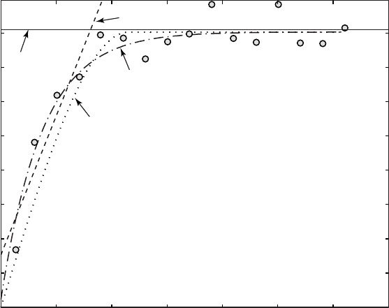
Another important question in variogram modeling is the intended
use of the model. In our case, the linear model at rst does not appear to
be appropriate (Fig. 7.21). Following a closer look, however, we can see that
the linear model ts reasonably well over the rst three lags. is can be
su cient if we use the variogram model only for kriging, because in krig-
ing the nearby points are the most important points for the estimate (see
discussion of kriging below). us, di erent variogram models with similar
ts close to the origin will yield similar kriging results when the sampling
points are regularly distributed. If the objective is to describe the spatial
246 7 SPATIAL DATA
Distance between observations
Semivariance
Population
variance
Spherical model
Exponential model
Linear model
0.1
0.2
0.3
0.4
0.5
0.6
0.7
0.8
0
0 20406080100120140
Fig. 7.21 Variogram estimator (gray circles), population variance (solid line), and spherical,
exponential, and linear models (dotted and dashed lines).
structures then the situation is quite di erent. It then becomes important to
nd a model that is suitable over all lags, and to accurately determine the sill
and the range. A collection of geological case studies in Rendu and Readdy
(1982) show how process knowledge and variography can be interlinked.
Good guidelines for variogram modeling are provided by Gringarten and
Deutsch (2001) and Webster and Oliver (2001).
We will now brie y discuss a number of other aspects of variography:
• Sample size – As in any statistical procedure, as large a sample as pos-
sible is required in order to obtain a reliable estimate. For variography
it is recommended that the number of samples should be in excess of
100 to 150 (Webster and Oliver 2001). For smaller sample numbers a
maximum likelihood variogram should be computed (Pardo-Igúzquiza
and Dowd 1997).
• Sampling design – In order to obtain a good estimation close to the ori-

7.11 GEOSTATISTICS AND KRIGING (BY R. GEBBERS) 247
7 SPATIAL DATA
gin of the variogram, the sampling design should include observations
over small distances. is can be achieved by means of a nested design
(Webster and Oliver 2001). Other possible designs have been evaluated
by Olea (1984).
• Anisotropy – us far we have assumed that the structure of spatial
correlation is independent of direction. We have calculated omnidirec-
tional variograms ignoring the direction of the separation vector h. In
a more thorough analysis, the variogram should be discretized not only
in distance but also in direction (directional bins). Plotting directional
variograms, usually in four directions, we sometimes can observe dif-
ferent ranges ( geometric anisotropy), di erent scales ( zonal anisotropy),
and di erent shapes (indicating a trend). e treatment of anisotropy
requires a highly interactive graphical user interface, which is beyond
the scope of this book (see the so ware VarioWin by Panatier 1996).
Number of pairs and the lag interval• – When calculating the classical
variogram estimator it is recommended that more than 30 to 50 pairs
of points be used per lag interval (Webster and Oliver 2001). is is due
to the sensitivity to outliers. If there are fewer pairs, the lag interval
should be increased. e lag spacing does not necessarily need to be
uniform, but can be chosen individually for each distance class. It is also
possible to work with overlapping classes, in which case the lag width
( lag tolerance) must be de ned. However, increasing the lag width can
cause unnecessary smoothing, with a resulting loss of detail. e sepa-
ration distance and the lag width therefore must be chosen with care.
Another option is to use a more robust variogram estimator (Cressie
1993, Deutsch and Journel 1998).
Calculation of • separation distance – If the observations cover a large
area, for example more than 1,000 km
2
, spherical distances should be
calculated instead of Pythagorean distances from a planar Cartesian co-
ordinate system.
Kriging
We will now interpolate the observations onto a regular grid by ordinary
point kriging which is the most popular kriging method. Ordinary point
kriging uses a weighted average of the neighboring points to estimate the
value of an unobserved point: