Tong W. Wind Power Generation and Wind Turbine Design

Подождите немного. Документ загружается.

Fundamentals of Wind Energy 5

towards the poles and cold air with higher density ﬂ ows from the poles towards the

equator along the earth’s surface. Without considering the earth’s self-rotation and

the rotation-induced Coriolis force, the air circulation at each hemisphere forms a

single cell, deﬁ ned as the meridional circulation.

Second, the earth’s self-rotating axis has a tilt of about 23.5° with respect to its

ecliptic plane. It is the tilt of the earth’s axis during the revolution around the sun

that results in cyclic uneven heating, causing the yearly cycle of seasonal weather

changes.

Third, the earth’s surface is covered with different types of materials such as vegeta-

tion, rock, sand, water, ice/snow, etc. Each of these materials has different reﬂ ecting

and absorbing rates to solar radiation, leading to high temperature on some areas (e.g.

deserts) and low temperature on others (e.g. iced lakes), even at the same latitudes.

The fourth reason for uneven heating of solar radiation is due to the earth’s

topographic surface. There are a large number of mountains, valleys, hills, etc. on

the earth, resulting in different solar radiation on the sunny and shady sides.

2.2 Coriolis force

The earth’s self-rotation is another important factor to affect wind direction and

speed. The Coriolis force, which is generated from the earth's self-rotation, deﬂ ects

the direction of atmospheric movements. In the north atmosphere wind is deﬂ ected

to the right and in the south atmosphere to the left. The Coriolis force depends on

the earth’s latitude; it is zero at the equator and reaches maximum values at the

poles. In addition, the amount of deﬂ ection on wind also depends on the wind

speed; slowly blowing wind is deﬂ ected only a small amount, while stronger wind

deﬂ ected more.

In large-scale atmospheric movements, the combination of the pressure gradient

due to the uneven solar radiation and the Coriolis force due to the earth’s self-

rotation causes the single meridional cell to break up into three convectional cells

in each hemisphere: the Hadley cell, the Ferrel cell, and the Polar cell ( Fig. 1 ).

Each cell has its own characteristic circulation pattern.

In the Northern Hemisphere, the Hadley cell circulation lies between the equa-

tor and north latitude 30°, dominating tropical and sub-tropical climates. The hot

air rises at the equator and ﬂ ows toward the North Pole in the upper atmosphere.

This moving air is deﬂ ected by Coriolis force to create the northeast trade winds.

At approximately north latitude 30°, Coriolis force becomes so strong to balance

the pressure gradient force. As a result, the winds are defected to the west. The air

accumulated at the upper atmosphere forms the subtropical high-pressure belt and

thus sinks back to the earth’s surface, splitting into two components: one returns to

the equator to close the loop of the Hadley cell; another moves along the earth’s

surface toward North Pole to form the Ferrel Cell circulation, which lies between

north latitude 30° and 60°. The air circulates toward the North Pole along the

earth’s surface until it collides with the cold air ﬂ owing from the North Pole at

approximately north latitude 60°. Under the inﬂ uence of Coriolis force, the mov-

ing air in this zone is deﬂ ected to produce westerlies. The Polar cell circulation lies

between the North Pole and north latitude 60°. The cold air sinks down at the

6 Wind Power Generation and Wind Turbine Design

North Pole and ﬂ ows along the earth’s surface toward the equator. Near north lati-

tude 60°, the Coriolis effect becomes signiﬁ cant to force the airﬂ ow to southwest.

2.3 Local geography

The roughness on the earth’s surface is a result of both natural geography and

manmade structures. Frictional drag and obstructions near the earth’s surface gen-

erally retard with wind speed and induce a phenomenon known as wind shear. The

rate at which wind speed increases with height varies on the basis of local condi-

tions of the topography, terrain, and climate, with the greatest rates of increases

observed over the roughest terrain. A reliable approximation is that wind speed

increases about 10% with each doubling of height [ 4 ].

In addition, some special geographic structures can strongly enhance the wind

intensity. For instance, wind that blows through mountain passes can form moun-

tain jets with high speeds.

3 History of wind energy applications

The use of wind energy can be traced back thousands of years to many ancient

civilizations. The ancient human histories have revealed that wind energy was

discovered and used independently at several sites of the earth.

North Pole

South Pole

0º

30º

60º

Hadley cell

Ferrel cell

Polar cell

Equator

Trade winds

Westerlies

Polar easterlies

Figure 1: Idealized atmospheric circulations.

Fundamentals of Wind Energy 7

3.1 Sailing

As early as about 4000 B.C., the ancient Chinese were the ﬁ rst to attach sails to

their primitive rafts [5]. From the oracle bone inscription, the ancient Chinese

scripted on turtle shells in Shang Dynasty (1600 B.C.–1046 B.C.), the ancient

Chinese character “ ” (i.e., “⑰”, sail - in ancient Chinese) often appeared. In

Han Dynasty (220 B.C.–200 A.D.), Chinese junks were developed and used as

ocean-going vessels. As recorded in a book wrote in the third century [6], there

were multi-mast, multi-sail junks sailing in the South Sea, capable of carrying 700

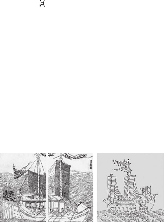
people with 260 tons of cargo. Two ancient Chinese junks are shown in Figure 2.

Figure 2(a) is a two-mast Chinese junk ship for shipping grain, quoted from the

famous encyclopedic science and technology book Exploitation of the works of

nature [7]. Figure 2(b) illustrates a wheel boat [8] in Song Dynasty (960–1279).

It mentioned in [9] that this type of wheel boats was used during the war between

Song and Jin Dynasty (1115–1234).

Approximately at 3400 BC, the ancient Egyptians launched their ﬁ rst sailing

vessels initially to sail on the Nile River, and later along the coasts of the

Mediterranean [ 5 ]. Around 1250 BC, Egyptians built fairly sophisticated ships to

sail on the Red Sea [ 9 ]. The wind-powered ships had dominated water transport

for a long time until the invention of steam engines in the 19th century.

3.2 Wind in metal smelting processes

About 300 BC, ancient Sinhalese had taken advantage of the strong monsoon

winds to provide furnaces with sufﬁ cient air for raising the temperatures inside

furnaces in excess of 1100°C in iron smelting processes. This technique was

capable of producing high-carbon steel [ 10 ].

Figure 2: Ancient Chinese junks (ships): (a) two-mast junk ship [ 7 ]; (b) wheel

boat [ 8 ] .

(a) (b)

8 Wind Power Generation and Wind Turbine Design

The double acting piston bellows was invented in China and was widely used

in metallurgy in the fourth century BC [ 11 ]. It was the capacity of this type of

bellows to deliver continuous blasts of air into furnaces to raise high enough tem-

peratures for smelting iron. In such a way, ancient Chinese could once cast several

tons of iron.

3.3 Windmills

China has long history of using windmills. The unearthed mural paintings from the

tombs of the late Eastern Han Dynasty (25–220 AD) at Sandaohao, Liaoyang City,

have shown the exquisite images of windmills, evidencing the use of windmills in

China for at least approximately 1800 years [ 12 ].

The practical vertical axis windmills were built in Sistan (eastern Persia) for

grain grinding and water pumping, as recorded by a Persian geographer in the

ninth century [ 13 ].

The horizontal axis windmills were invented in northwestern Europe in 1180s

[ 14 ]. The earlier windmills typically featured four blades and mounted on central

posts – known as Post mill. Later, several types of windmills, e.g. Smock mill,

Dutch mill, and Fan mill, had been developed in the Netherlands and Denmark,

based on the improvements on Post mill.

The horizontal axis windmills have become dominant in Europe and North

America for many centuries due to their higher operation efﬁ ciency and technical

advantages over vertical axis windmills.

3.4 Wind turbines

Unlike windmills which are used directly to do work such as water pumping or

grain grinding, wind turbines are used to convert wind energy to electricity. The

ﬁ rst automatically operated wind turbine in the world was designed and built by

Charles Brush in 1888. This wind turbine was equipped with 144 cedar blades

having a rotating diameter of 17 m. It generated a peak power of 12 kW to charge

batteries that supply DC current to lamps and electric motors [ 5 ].

As a pioneering design for modern wind turbines, the Gedser wind turbine was

built in Denmark in the mid 1950s [ 15 ]. Today, modern wind turbines in wind

farms have typically three blades, operating at relative high wind speeds for the

power output up to several megawatts.

3.5 Kites

Kites were invented in China as early as the ﬁ fth or fourth centuries BC [ 11 ]. A

famous Chinese ancient legalist Han Fei-Zi (280–232 BC) mentioned in his book

that an ancient philosopher Mo Ze (479–381 BC) spent three years to make a kite

with wood but failed after one-day ﬂ ight [ 16 ].

Fundamentals of Wind Energy 9

4 Wind energy characteristics

Wind energy is a special form of kinetic energy in air as it ﬂ ows. Wind energy can

be either converted into electrical energy by power converting machines or directly

used for pumping water, sailing ships, or grinding gain.

4.1 Wind power

Kinetic energy exists whenever an object of a given mass is in motion with a trans-

lational or rotational speed. When air is in motion, the kinetic energy in moving

air can be determined as

Emu=

(1)

where m is the air mass and u

–

is the mean wind speed over a suitable time period.

The wind power can be obtained by differentiating the kinetic energy in wind with

respect to time, i.e.:

Pmu



(2)

However, only a small portion of wind power can be converted into electrical

power. When wind passes through a wind turbine and drives blades to rotate, the

corresponding wind mass ﬂ owrate is

mAur=



(3)

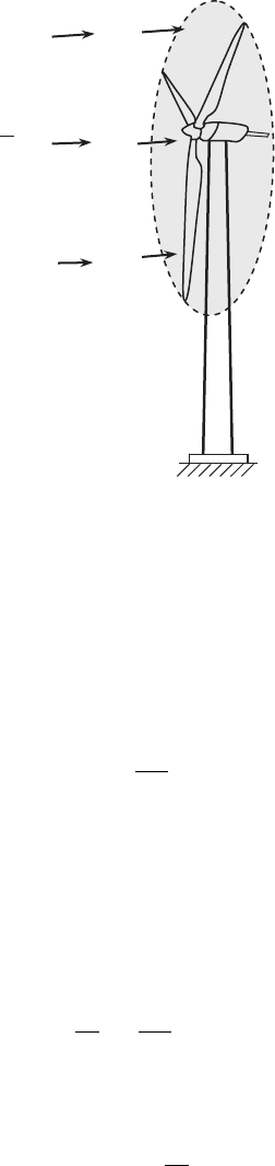
where r is the air density and A is the swept area of blades, as shown in Fig. 3 .

Substituting (3) into (2), the available power in wind P

can be expressed as

PAur=

(4)

An examination of eqn (4) reveals that in order to obtain a higher wind power, it

requires a higher wind speed, a longer length of blades for gaining a larger swept

area, and a higher air density. Because the wind power output is proportional to the

cubic power of the mean wind speed, a small variation in wind speed can result in

a large change in wind power.

4.1.1 Blade swept area

As shown in Fig. 3 , the blade swept area can be calculated from the formula:

(

)

(

)

2Alrr llrpp

⎡⎤

=+−=+

⎣⎦

(5)

10 Wind Power Generation and Wind Turbine Design

where l is the length of wind blades and r is the radius of the hub. Thus, by doubling

the length of wind blades, the swept area can be increased by the factor up to 4.

When l >> 2 r , A ≈ p l

4.1.2 Air density

Another important parameter that directly affects the wind power generation is the

density of air, which can be calculated from the equation of state:

r =

(6)

where p is the local air pressure, R is the gas constant (287 J/kg-K for air), and T

is the local air temperature in K.

The hydrostatic equation states that whenever there is no vertical motion, the

difference in pressure between two heights is caused by the mass of the air layer:

ddpgzr=−

(7)

where g is the acceleration of gravity. Combining eqns (6) and (7), yields

pRT

=−

( 8 )

The acceleration of gravity g decreases with the height above the earth’s

surface z :

⎛⎞

=−

⎜⎟

⎝⎠

(9)

Figure 3: Swept area of wind turbine blades .

Fundamentals of Wind Energy 11

where g

is the acceleration of gravity at the ground and D is the diameter of the

earth. However, for the acceleration of gravity g , the variation in height can be

ignored because D is much larger than 4 z .

In addition, temperature is inversely proportional to the height. Assume that d T /

d z = c , it can be derived that

gcR

−

⎛⎞

⎜⎟

⎝⎠

(10)

where p

and T

are the air pressure and temperature at the ground, respectively.

Combining eqns (6) and (10), it gives

(/ 1) (/ 1)

gcR gcR

Tcz

rr r

−+ −+

⎛⎞ ⎛ ⎞

==+

⎜⎟ ⎜ ⎟

⎝⎠ ⎝ ⎠

(11)

This equation indicates that the density of air decreases nonlinearly with the height

above the sea level.

4.1.3 Wind power density

Wind power density is a comprehensive index in evaluating the wind resource

at a particular site. It is the available wind power in airflow through a per-

pendicular cross-sectional unit area in a unit time period. The classes of

wind power density at two standard wind measurement heights are listed in

Table 1 .

Some of wind resource assessments utilize 50 m towers with sensors installed at

intermediate levels (10 m, 20 m, etc.). For large-scale wind plants, class rating of

4 or higher is preferred.

Table 1: Classes of wind power density [ 17 ].

Wind power

class

10 m height 50 m height

Wind power

density (W/m

)

Mean wind

speed (m/s)

Wind power

density (W/m

)

Mean wind

speed (m/s)

1 <100 <4.4 <200 <5.6

2 100–150 4.4–5.1 200–300 5.6–6.4

3 150–200 5.1–5.6 300–400 6.4–7.0

4 200–250 5.6–6.0 400–500 7.0–7.5

5 250–300 6.0–6.4 500–600 7.5–8.0

6 300–350 6.4–7.0 600–800 8.0–8.8

7 >400 >7.0 >800 >8.8

12 Wind Power Generation and Wind Turbine Design

4.2 Wind characteristics

Wind varies with the geographical locations, time of day, season, and height above

the earth’s surface, weather, and local landforms. The understanding of the wind

characteristics will help optimize wind turbine design, develop wind measuring

techniques, and select wind farm sites.

4.2.1 Wind speed

Wind speed is one of the most critical characteristics in wind power generation.

In fact, wind speed varies in both time and space, determined by many factors

such as geographic and weather conditions. Because wind speed is a random

parameter, measured wind speed data are usually dealt with using statistical

methods.

The diurnal variations of average wind speeds are often described by sine waves.

As an example, the diurnal variations of hourly wind speed values, which are the

average values calculated based on the data between 1970 and 1984, at Dhahran,

Saudi Arabia have shown the wavy pattern [ 18 ]. The wind speeds are higher in

daytime and the maximum speed occurs at about 3 p.m., indicating that the day-

time wind speed is proportional to the strength of sunlight. George et al. [ 19 ]

reported that wind speed at Lubbock, TX is near constant during dark hours, and

follows a curvilinear pattern during daylight hours. Later, George et al. [ 20 ] have

demonstrated that diurnal wind patterns at ﬁ ve locations in the Great Plains follow

a pattern similar to that observed in [ 19 ].

Based on the wind speed data for the period 1970–2003 from up to 66 onshore

sites around UK, Sinden [ 21 ] has concluded that monthly average wind speed is

inversely propositional to the monthly average temperature, i.e. it is higher in the

winter and lower in the summer. The maximum wind speed occurs in January and

the minimum in August. Hassanm and Hill have reported that the month-to-month

variation of mean wind speed values over the period of 1970–1984 at Dhahran,

Saudi Arabia has shown the wavy pattern [ 13 ]. However, because the variation in

temperature at Dhahran is small over the whole year, there is no a clear correlation

between wind speed and temperatures.

The year-to-year variation of yearly mean wind speeds depends highly

on selected locations and thus there is no common correlation to predict it.

For instance, except for several years, the annual mean wind speeds decrease

all the way from 1970 to 1983 at Dhahran, Saudi Arabia [ 18 ]. In UK, this

variation displays in a more ﬂ uctuated matter for the period 1970–2003 [ 21 ].

Similarly, a signiﬁ cant variation in the annual mean wind speed over 20-year

period (1978–1998) is reported in [ 22 ], with maximum and minimum values

ranging from less than 7.8 to nearly 9.2 m/s. The long-term wind data (1978–

2007) obtained from automated synoptic observation system of meteorologi-

cal observatories were analyzed and reported by Ko et al. [ 23 ]. The results

show that ﬂ uctuation in yearly average wind speed occurs at the observed sites;

it tends to slightly decrease at Jeju Island, while the other two sites have

random trends.

Fundamentals of Wind Energy 13

4.2.2 Weibull distribution

The variation in wind speed at a particular site can be best described using the

Weibull distribution function [ 24 ], which illustrates the probability of different

mean wind speeds occurring at the site during a period of time. The probability

density function of a Weibull random variable u

–

is:

(

)

exp 0

ku u

fuk

ll l

−

⎧

⎛⎞

⎛⎞ ⎛⎞

−≥

⎪

⎜⎟

⎜⎟ ⎜⎟

⎝⎠ ⎝⎠

⎨

⎝⎠

⎪

⎩

(12)

where l is the scale factor which is closely related to the mean wind speed and k

is the shape factor which is a measurement of the width of the distribution. These

two parameters can be determined from the statistical analysis of measured wind

speed data at the site [ 25 ]. It has been reported that Weibull distribution can give

good ﬁ ts to observed wind speed data [ 26 ]. As an example, the Weibull distribu-

tions for various mean wind speeds are displayed in Fig. 4 .

4.2.3 Wind turbulence

Wind turbulence is the ﬂ uctuation in wind speed in short time scales, especially

for the horizontal velocity component. The wind speed u ( t ) at any instant time t

can be considered as having two components: the mean wind speed u

–

and the

instantaneous speed ﬂ uctuation u ′( t ), i.e.:

(

)

(

)

ut u u t=+

′

(13)

15 20 25 30 35

u = 2 m/s

6 m/s

10 m/s

16 m/s

20 m/s

Wind Speed (m/s)

Probability (%)

Figure 4: Weibull distributions for various mean wind speeds.

14 Wind Power Generation and Wind Turbine Design

Wind turbulence has a strong impact on the power output ﬂ uctuation of wind

turbine. Heavy turbulence may generate large dynamic fatigue loads acting on

the turbine and thus reduce the expected turbine lifetime or result in turbine

failure.

In selection of wind farm sites, the knowledge of wind turbulence intensity is

crucial for the stability of wind power production. The wind turbulence intensity I

is deﬁ ned as the ratio of the standard deviation s

to the mean wind velocity u

–

(14)

where both s

and u

–

are measured at the same point and averaged over the same

period of time.

4.2.4 Wind gust

Wind gust refers to a phenomenon that a wind blasts with a sudden increase

in wind speed in a relatively small interval of time. In case of sudden turbulent

gusts, wind speed, turbulence, and wind shear may change drastically. Reducing

rotor imbalance while maintaining the power output of wind turbine generator

constant during such sudden turbulent gusts calls for relatively rapid changes of

the pitch angle of the blades. However, there is typically a time lag between the

occurrence of a turbulent gust and the actual pitching of the blades based upon

dynamics of the pitch control actuator and the large inertia of the mechanical com-

ponents. As a result, load imbalances and generator speed, and hence oscillations

in the turbine components may increase considerably during such turbulent gusts,

and may exceed the maximum prescribed power output level [ 27 ]. Moreover, sud-

den turbulent gusts may also signiﬁ cantly increase tower fore-aft and side-to-side

bending moments due to increase in the effect of wind shear.

To ensure safe operation of wind farms, wind gust predictions are highly desired.

Several different gust prediction methods have been proposed. Contrary to most

techniques used in operational weather forecasting, Brasseur [ 29 ] developed a new

wind gust prediction method based on physical consideration. In another study

[ 30 ], it reported that using a gust factor, which is deﬁ ned as peak gust over the

mean wind speed, could well forecast wind gust speeds. These results are in agree-

ment with previous work by other investigators [ 31 ].

4.2.5 Wind direction

Wind direction is one of the wind characteristics. Statistical data of wind direc-

tions over a long period of time is very important in the site selection of wind farm

and the layout of wind turbines in the wind farm.

The wind rose diagram is a useful tool of analyzing wind data that are related to

wind directions at a particular location over a speciﬁ c time period (year, season,

month, week, etc.). This circular diagram displays the relative frequency of wind

directions in 8 or 16 principal directions. As an example shown in Fig. 5 , there are

16 radial lines in the wind rose diagram, with 22.5° apart from each other. The

length of each line is proportional to the frequency of wind direction. The frequency