Tennick A. Practical PowerPivot & DAX Formulas for Excel 2010
Подождите немного. Документ загружается.


374 Practical PowerPivot & DAX Formulas for Excel 2010
is is MDX, not DAX! MDX is a query language for SSAS cubes—it’s talking
directly to the hidden cube, called PowerPivot Data, behind PowerPivot. MDX
is beyond the scope of this book—if you are interested, please refer to my book,
Practical MDX Queries for Microsoft SQL Server Analysis Services 2008 (McGraw-
Hill/Professional, 2010).
5. Edit the MDX so it looks like the following:
Topcount
(
{
([Products].[Category].&[Beverages]),
([Products].[Category].&[Condiments]),
([Products].[Category].&[Confections]),
([Products].[Category].&[Dairy Products]),
([Products].[Category].&[Grains/Cereals]),
([Products].[Category].&[Meat/Poultry]),
([Products].[Category].&[Produce]),
([Products].[Category].&[Seafood])
},
3,
[Measures].[Sales]
)
ere are a few changes in this MDX. ([Products].[Category].[All])
has been removed—this is going to remove Grand Total from the column in the
pivot table. Before the first curly bracket, Topcount ( has been added. After
the last curly bracket, , 3, [Measures].[Sales] ) has been added. is is
assuming you have a measure called Sales (=SUM('Order Details'[Sales
Amount])) that sums up Sales Amount.
6. You may want to click Test MDX before clicking OK. Your set is visible in the
PowerPivot Field List, under Sets. Your pivot table should look like Figure 12-30.
e rows are showing the top three categories for sales. e third one, in my
example, is Meat/Poultry.
Figure 12-30 A predefined set
Chapter 12: A Few Ideas: PowerPivot and DAX Solutions 375
7. Remove Sales from Values and add Quantity from Order Details. You should still
see the same three categories. However, these are the top three by sales, not by
quantity. In fact, Meat/Poultry is only number seven by quantity. You can prove this
by replacing the set in Row Labels with Category from Products again and sorting
largest to smallest on quantity. This is really quite powerful stuff! You can display
rows (or columns) with a particular measure, but with the criteria determined by
a non-visible measure. A little MDX gives you lots of control. You could do this
through the GUI (Row Labels, Value Filters, Top 10… and choose a different
measure from the current measure)—however, it involves a bit of work every time.
A set can simply be reused as and when required. The following example would
be a little bit more difficult through the GUI—it shows the second and third top
categories by sales, no matter which measure is being displayed:
Except
(
topcount
(
{
([Products].[Category].&[Beverages]),
([Products].[Category].&[Condiments]),
([Products].[Category].&[Confections]),
([Products].[Category].&[Dairy Products]),
([Products].[Category].&[Grains/Cereals]),
([Products].[Category].&[Meat/Poultry]),
([Products].[Category].&[Produce]),
([Products].[Category].&[Seafood])
},
3,
[Measures].[Sales]),
topcount
(
{
([Products].[Category].&[Beverages]),
([Products].[Category].&[Condiments]),
([Products].[Category].&[Confections]),
([Products].[Category].&[Dairy Products]),
([Products].[Category].&[Grains/Cereals]),
([Products].[Category].&[Meat/Poultry]),
([Products].[Category].&[Produce]),
([Products].[Category].&[Seafood])},
1,
[Measures].[Sales]
)
)
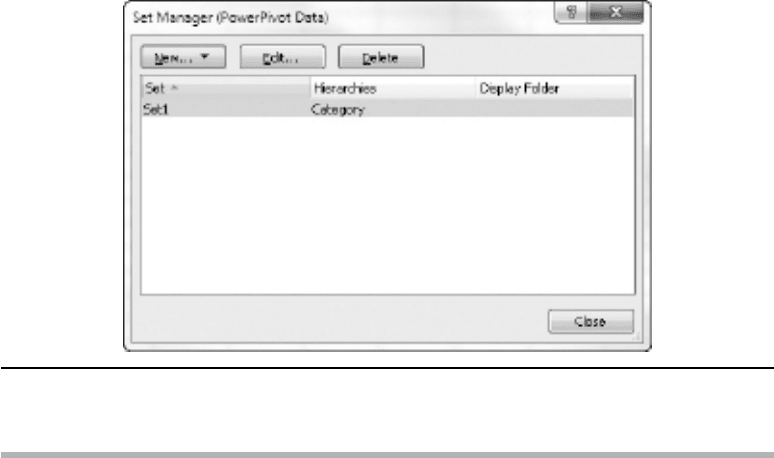
8. If you want to change a set, click Fields, Items, & Sets again. This time, choose
Manage Sets from the drop-down menu. This opens the Set Manager dialog, as
shown in Figure 12-31. Select your set and click Edit to see the Modify Set dialog.
This dialog is the same as the New Set dialog shown earlier in Figure 12-28.

376 Practical PowerPivot & DAX Formulas for Excel 2010
PowerPivot Without Pivot Table Data
So far, this book has used pivot tables (and occasionally pivot charts) to display data from
the PowerPivot model. However, you don’t have to use pivot reports to display data. This
section shows how to visualize PowerPivot model data without doing so in a pivot table.
There are a couple of reasons why you might want to do this. One, you want to create
your own custom front end in an Excel worksheet. Two, you might want to manipulate
the data further with functions from Excel’s formidable arsenal of functions. There are
many ways to access PowerPivot data without a pivot table. You could use VBA in Excel,
or, perhaps, create an SSRS report on a PowerPivot model published to SharePoint.
In this section, two alternative approaches are considered. One exploits the Excel
GETPIVOTDATA() function, and the other uses the Excel CUBE() family of functions.
GETPIVOTDATA()
Maybe this one is cheating slightly. There is still a pivot table, except it might be on a
separate worksheet—which, optionally, you can hide. There is an Excel function called
GETPIVOTDATA(). This function extracts data from a pivot table. You place the function
in a cell that is away from the pivot table, or, better, on a separate worksheet. Fortunately,
this function is self-generating. From a cell, type = in the Excel formula bar, then click on
a value in the data area of a pivot table, then press enter. The GETPIVOTDATA() syntax
to reference the data in the pivot table is generated. Here’s an example:
=GETPIVOTDATA("[Measures].[Sum of Quantity]",$A$1,
"[Products].[Category]","[Products].[Category].&[Beverages]")
Figure 12-31 Set Manager dialog
Chapter 12: A Few Ideas: PowerPivot and DAX Solutions 377
The first parameter is a reference to the measure you wish to return. The second
parameter locates the pivot table you wish to reference. Then you can have any number
of parameters that provide the coordinates for the data. Here, it’s going to show the
sales for Beverages.
If you want to write this function by hand, the syntax to reference a pivot table
on a different worksheet is slightly different. Following is the same example, but it’s
referencing a pivot table in Sheet2 (please note the addition of Sheet2!):
=GETPIVOTDATA("[Measures].[Sum of Quantity]",Sheet2!$A$1,
"[Products].[Category]","[Products].[Category].&[Beverages]")
You can use GETPIVOTDATA() to calculate BI answers that are not so easy through
the pivot table GUI or DAX. For example, you might want to show the sales of two
products from two separate product categories as a percentage of the two product
categories combined.
Should GETPIVOTDATA() not self-generate, it may be turned off. To check this, click
File | Options | Formulas and look at the setting for Use GetPivotData functions for
PivotTable references. Alternatively, check the setting for Generate GetPivotData in the
Options drop-down menu in the PivotTable group of the PivotTable Tools/Options ribbon.
CUBE() Functions
This time, the example uses the Excel CUBE() functions. If these are new to you, here
are the step-by-step instructions:
1. Add a new pivot table to an existing worksheet and position it at $A$1. If you
add it to a new worksheet it will be positioned at cell $B$3. Should you do the
latter, please adjust all cell references in these step-by-step instructions—you will need
to move every reference across by one column and down by two rows. Click in the
empty pivot table to activate the PowerPivot Field List. Add Year to the Slicers
Horizontal drop-zone, and Year again to the Report Filter drop-zone. Verify
the Report Filter position as A9:B9—if not, change the reference to $B$9 that
appears in step 6.
2. Click in cell C9 and enter the following formula:
=CUBEMEMBER("PowerPivot Data","[Measures].[Sales]","Sales")
is assumes you have a measure called Sales that sums the Sales Amount
(=SUM('Order Details'[Sales Amount])). e first parameter is the
connection to PowerPivot—you can check this name by going through PivotTable
Tools/Options | Data | Change Data Source | Connection Properties. is opens
the Connection Properties dialog. e connection name is at the top of this
dialog. e full connection string is on the Definition tab. e second parameter
of our formula is the measure to show, and the third parameter is a caption.
378 Practical PowerPivot & DAX Formulas for Excel 2010
3.
Click in cell A10. Enter the following formula:
=CUBESET("PowerPivot Data","[Products].[Category].[All].Children",
"Category")
is is using MDX to create the children of the All member of Category (for
example, Beverages). e third parameter is a caption. Further parameters, not
shown here, allow you to specify a sort order and a measure to sort on. For a
full discussion of the CUBE() functions, you are referred to Excel Help. To
understand the CUBE() functions, it helps to have a little knowledge of MDX.
4. Click in cell A11 and enter the following formula:
=IFERROR(CUBERANKEDMEMBER("PowerPivot Data",$A$10,ROW(A1)),"")
is formula is going to retrieve the first product category, Beverages, from the set
defined in cell A10. ROW(A1) returns 1, but you can’t use 1, as this cell is going to
be copied down and we want it to return the second category, then the third, and
so on. Hard-coded numerals are, well, hard-coded. e IFERROR() function is to
suppress nonexistent categories, if we copy too far down.
5. Copy cell A11 from A12 to about A20. You should see a total of eight categories
(including Beverages). You may want to widen column A, to display the complete
names of the categories.
6. Click in cell B11 and enter this formula:
=IFERROR(CUBEVALUE("PowerPivot Data",$A11,$B$9,$C$9),"")
is function is referencing Beverages (A11) and the report filter on Year (B9)
and the Sales measure (C9). In other words, it’s returning the Sales for Beverages
for the current filter on Year. You may have to widen the column for the number
to display in non-scientific format.
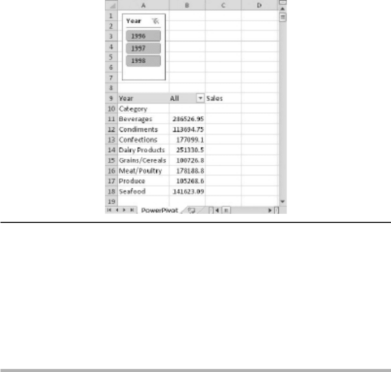
7. Copy B11 from B12 to about B20. Hopefully, you can see the sales for each
category. Experiment with the Year filter. My result is shown in Figure 12-32.
8. Instead of a Report Filter on Year, you may prefer to use the Year slicer. It’s also
probably overkill to have Year in both a Report Filter and a slicer, as here. If you
do reference the slicer, the formula for B11 might look like this:
=IFERROR(CUBEVALUE("PowerPivot Data",$A11,Slicer_Year,$C$9),"")
Please note the third parameter of CUBEVALUE() now references the slicer. To
verify the name of a slicer, open the Slicer Settings dialog and check the Name
to use in formulas entry. e slicer name is not enclosed in quotes. In addition,
this example formula assumes that Excel column and row references are still
valid. If you want to use a slicer, it’s probably a good idea to add the slicer before

Chapter 12: A Few Ideas: PowerPivot and DAX Solutions 379
you start using cell references. Please note that adding or removing entries in the
PowerPivot Field List drop-zones may invalidate any cell references you may
have—or lose your CUBE() function formulas altogether. If you are interested,
you can view the MDX behind CUBERANKEDMEMBER() and CUBEMEMBER(). To
do so, view the Immediate Window in VBA (press alt-f), type the following
command, and press enter:
? ActiveCell.MDX
Self-Joins
Self-joins are not supported in PowerPivot. Here is the SQL to denormalize the
Northwind Employees table:
select E.EmployeeID, E.LastName, E.FirstName,
M.LastName + ', ' + M.FirstName as Manager from employees as E
left outer join employees as M
on E.ReportsTo = M.EmployeeID
Now you can analyze sales by employee by manager. This example is also in Appendix A
about SQL queries for PowerPivot, but included here in case you miss it in Appendix A.
Figure 12-32 PowerPivot data not in pivot table

380 Practical PowerPivot & DAX Formulas for Excel 2010
Data Mining
Appendix C is an introduction to writing DMX queries for PowerPivot. A DMX query
allows you to return data from an SSAS data mining model or mining structure. There is
another way to use data mining data without having to write DMX. If you download the
Data Mining Add-in for Excel, you can generate data mining data in a worksheet with
no writing of DMX yourself required. You can then import or link the worksheet into
PowerPivot. You have to use the Table Tools/Analyze ribbon and not the Data Mining
ribbon—the latter ribbon uses SSAS graphical interfaces and does not create data in a
worksheet. The add-in is downloadable from www.sqlserverdatamining.com. As of this
writing, only the Excel 2007 version was available, but it should work with Excel 2010
(32-bit only).
SSRS
Very early in this book, there was a discussion of importing data from an SSRS report
into a PowerPivot model. You can also export from an SSRS report into a PowerPivot
model—use the Export to Data Feed button, while viewing a report in Report
Manager, to do so. You can even reverse the whole process and base an SSRS report
on a PowerPivot model. To do this, you must first have published your PowerPivot for
Excel model to PowerPivot for SharePoint.
SharePoint
If you want to share your PowerPivot for Excel models and pivot reports, you can
publish from Excel to SharePoint. Go through File | Save & Send | Save to SharePoint
to accomplish this. Naturally, for this to work you have to have SharePoint (2010 not 2007),
and that means a 64-bit SharePoint server. In addition, you will need SQL Server 2008
R2 and SSAS installed in SharePoint-integrated mode. Further steps involve enabling
PowerPivot for SharePoint and Excel Services within SharePoint administration.
PowerPivot for SharePoint uses SSAS 2008 R2 in integrated mode to look after the data.
Excel Services is responsible for rendering the workbook containing the PowerPivot
pivot reports for thin clients, such as Internet Explorer.
Is It Really a Cube?
I hesitated before adding this topic—how to see PowerPivot as a cube. Please do not
try this on an important PowerPivot model—if you change the cube design, you can
easily invalidate the model! Copy an Excel workbook containing a PowerPivot model.
Change the file extension from .xlsx to .zip. Unzip the zip file. In the folder called xl,
open the folder called customData. In this last folder is a file called item1.data—this is

Chapter 12: A Few Ideas: PowerPivot and DAX Solutions 381
the cube data behind PowerPivot. Copy item1.data to your SSAS backup directory and
change the file extension from .data to .abf (Analysis Services backup file). You can now
restore the backup to an SSAS database and cube—this only works with SSAS 2008
R2 in SharePoint-integrated mode (or in-memory VertiPaq mode).
How Old Is Nancy?
Many years ago, when people learned SQL for SQL Server with the Northwind
database, there was a classic query. It was called “Nancy married the CEO.” The idea
was to practice the SQL Update statement and change Nancy’s Title from Ms. to Mrs.
and her LastName from Davolio to Fuller. If you look at the self-join on the Employees
just above, Andrew Fuller has no manager—he’s the boss!
This, possibly, will be the DAX equivalent of that SQL classic. It’s called “How old is
Nancy.” Here’s the DAX formula to work out age (on the Northwind Employees table):
=YEAR(TODAY())-YEAR(Employees[BirthDate])
It seems a shame to end a book on something that doesn’t always give the correct
result—that is, if you try it any time of the year apart from later on in December. Here’s
the one that does work (both results are shown in Figure 12-33):
=IF(MONTH(TODAY())>MONTH(Employees[BirthDate]),
YEAR(TODAY())-YEAR(Employees[BirthDate]),
IF(AND(MONTH(TODAY())=MONTH(Employees[BirthDate]),
DAY(TODAY())>=DAY(Employees[BirthDate])),
YEAR(TODAY())-YEAR(Employees[BirthDate]),
(YEAR(TODAY())-YEAR(Employees[BirthDate]))-1))
Can you find a more elegant way of calculating Nancy’s age?
That’s it, some nice DAX to finish. Well done if you got this far! Finito (oh, maybe
apart from just three appendixes).
Figure 12-33 How old is Nancy?
This page intentionally left blank

Appendixes: Queries
for PowerPivot
Part IV
