Stewart J. Calculus
Подождите немного. Документ загружается.

112
In this chapter we begin our study of differential calculus, which is concerned with how
one quantity changes in relation to another quantity. The central concept of differential
calculus is the derivative, which is an outgrowth of the velocities and slopes of tangents
that we considered in Chapter 2. After learning how to calculate derivatives, we use
them to solve problems involving rates of change and the approximation of functions.
DERIVATIVES
3
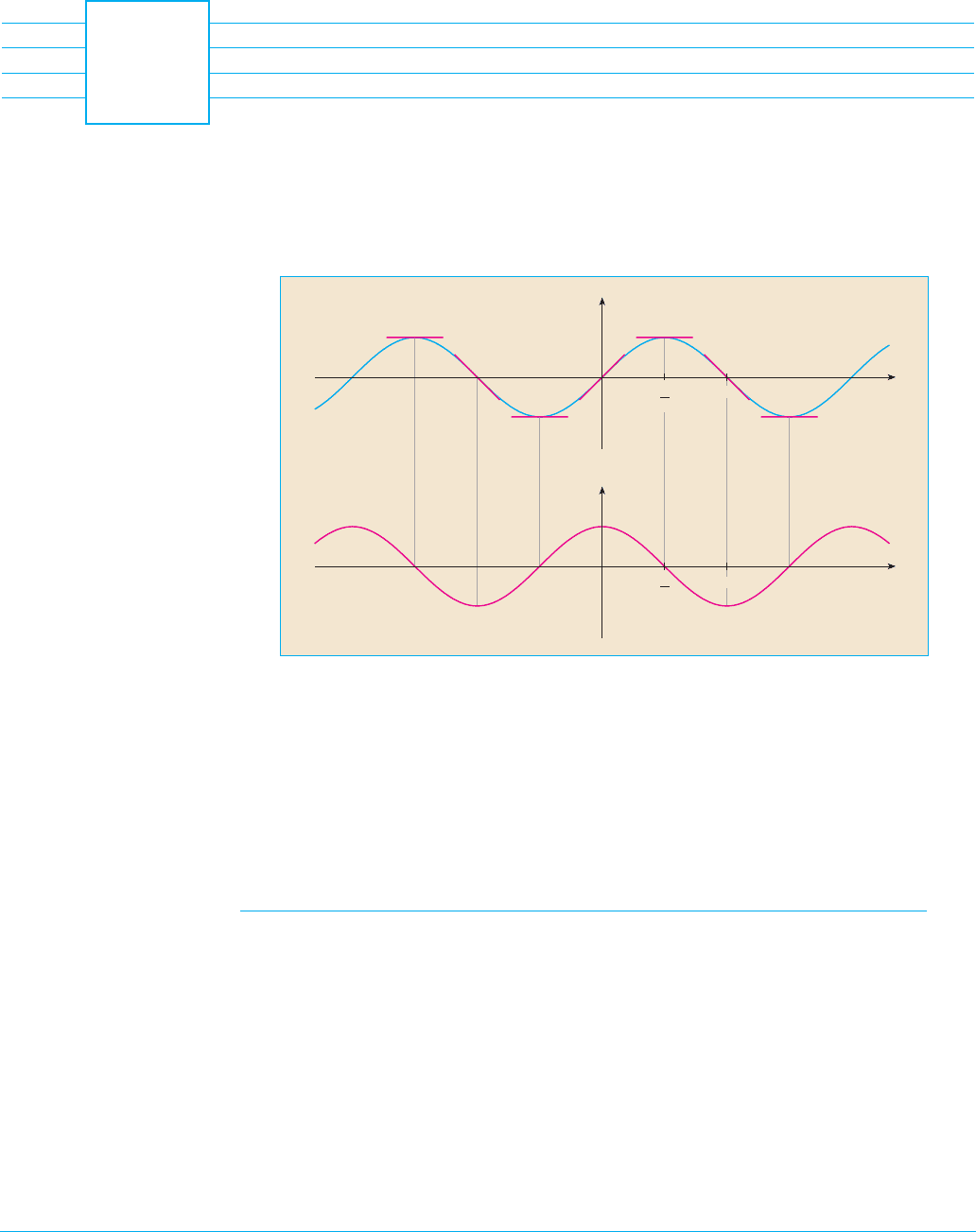
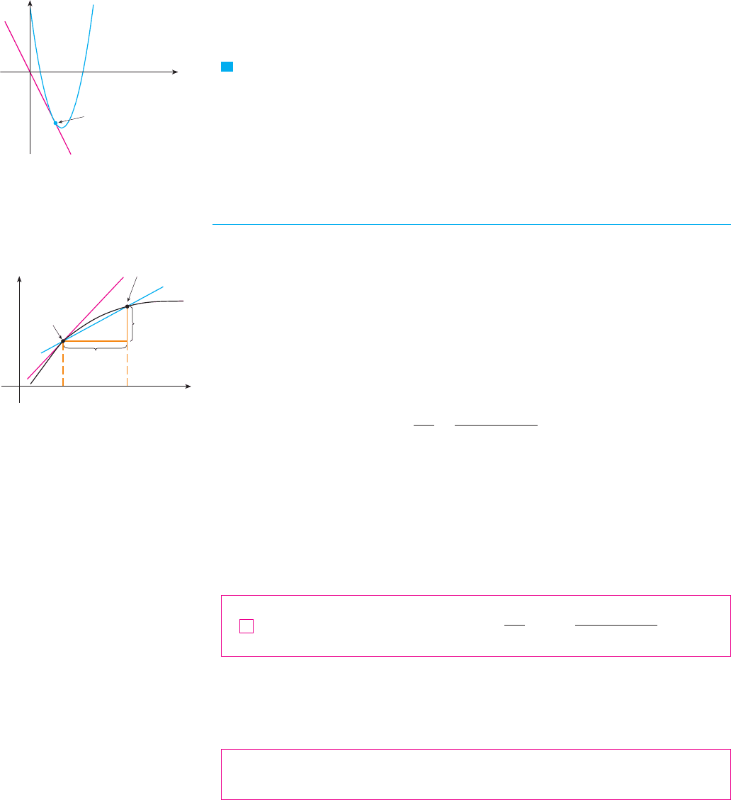
By measuring slopes at points on the sine curve,
we get strong visual evidence that the derivative
of the sine function is the cosine function.
x
ƒ=y= sin x
0
x
y
y
fª(xy= )
0
π
2
m=1 m=_1
m=0
π
2
π
π
DERIVATIVES AND RATES OF CHANGE
The problem of finding the tangent line to a curve and the problem of finding the velocity
of an object both involve finding the same type of limit, as we saw in Section 2.1. This spe-
cial type of limit is called a derivative and we will see that it can be interpreted as a rate
of change in any of the sciences or engineering.
TANGENTS
If a curve has equation and we want to find the tangent line to at the point
, then we consider a nearby point , where , and compute the slope
of the secant line :
Then we let approach along the curve by letting approach . If approaches a
number , then we define the tangent t to be the line through with slope . (This
amounts to saying that the tangent line is the limiting position of the secant line as
approaches . See Figure 1.)
DEFINITION The tangent line to the curve at the point is
the line through with slope
provided that this limit exists.
In our first example we confirm the guess we made in Example 1 in Section 2.1.
EXAMPLE 1 Find an equation of the tangent line to the parabola at the
point .
SOLUTION Here we have and , so the slope is
Using the point-slope form of the equation of a line, we find that an equation of the
tangent line at is
M
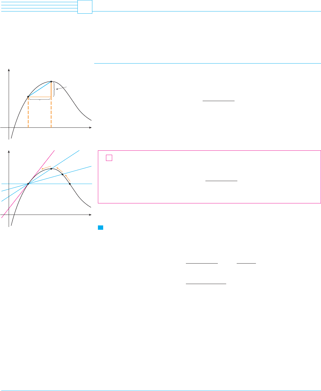
We sometimes refer to the slope of the tangent line to a curve at a point as the slope of
the curve at the point. The idea is that if we zoom in far enough toward the point, the curve
looks almost like a straight line. Figure 2 illustrates this procedure for the curve in y ! x
2
y ! 2x ! 1ory ! 1 ! 2!x ! 1"
!1, 1"
! lim
x l1
!x " 1" ! 1 " 1 ! 2
! lim
x l1
!x ! 1"!x " 1"
x ! 1
m ! lim
x l1
f !x" ! f !1"
x ! 1
! lim
x l1
x
2
! 1
x ! 1
f !x" ! x
2
a ! 1
P!1, 1"
y ! x
2
V
m ! lim
x l a
f !x" ! f !a"
x ! a
P
P!a, f !a""y ! f !x"
1
P
QPQ
mPm
m
PQ
axCPQ
m
PQ
!
f !x" ! f !a"
x ! a
PQ
x " aQ!x, f !x""P!a, f !a""
Cy ! f !x"C
3.1
113
N Point-slope form for a line through the
point with slope :
y ! y
1
! m!x ! x
1
"
m!x
1
, y
1
"
F I G U R E 1
0
x
y
P
t
Q
Q
Q
0
x
y
a x
P
{
a,f(a)
}
ƒ-f(a)
x-a
Q
{
x,ƒ
}
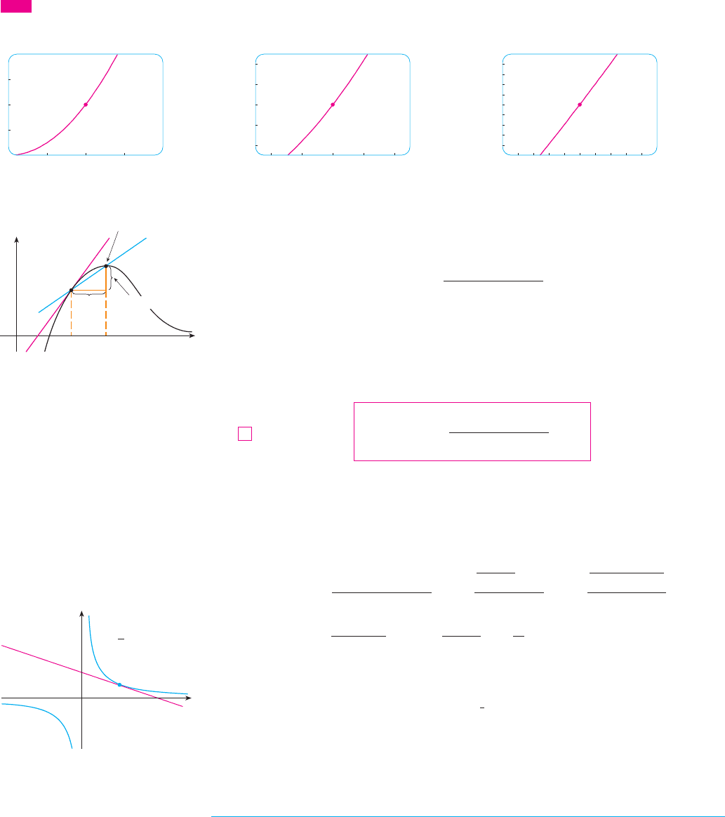
Example 1. The more we zoom in, the more the parabola looks like a line. In other words,
the curve becomes almost indistinguishable from its tangent line.
There is another expression for the slope of a tangent line that is sometimes easier to
use. If , then and so the slope of the secant line is
(See Figure 3 where the case is illustrated and is to the right of . If it happened
that , however, would be to the left of .)
Notice that as approaches , approaches (because ) and so the expres-
sion for the slope of the tangent line in Definition 1 becomes
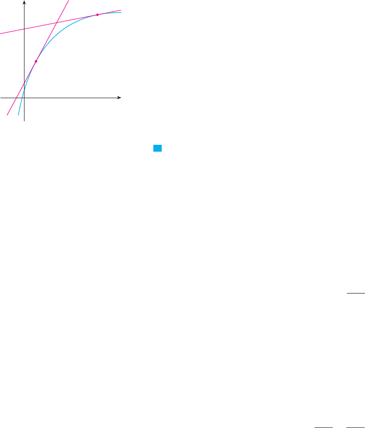
EXAMPLE 2 Find an equation of the tangent line to the hyperbola at the
point .
SOLUTION Let . Then the slope of the tangent at is
Therefore an equation of the tangent at the point is
which simplifies to
The hyperbola and its tangent are shown in Figure 4.
M
VELOCITIES
In Section 2.1 we investigated the motion of a ball dropped from the CN Tower and defined
its velocity to be the limiting value of average velocities over shorter and shorter time
periods.
x " 3y ! 6 ! 0
y ! 1 ! !
1
3
!x ! 3"
!3, 1"
! lim
h
l
0
!h
h!3 " h"
! lim
h
l
0
!
1
3 " h
! !
1
3
! lim
h
l
0
3
3 " h
! 1
h
! lim
h
l
0
3 ! !3 " h"
3 " h
h
m ! lim
h
l
0
f !3 " h" ! f !3"
h
!3, 1"f !x" ! 3#x
!3, 1"
y ! 3#x
m ! lim
h l 0
f !a " h" ! f !a"
h
2
h ! x ! a0hax
PQh
#
0
PQh $ 0
m
PQ
!
f !a " h" ! f !a"
h
PQx ! a " hh ! x ! a
F I G U R E 2 Zooming in toward the point (1,1) on the parabola y=≈
(1,1)
2
0
2
(1,1)
1.5
0.5
1.5
(1,1)
1.1
0.9
1.1
114
|| ||
CHAPTER 3 DERIVATIVES
Visual 3.1 shows an animation of
Figure 2.
TE C
F I G U R E 3
0
x
y
a
a+h
P
{
a,f(a)
}
h
Q
{
a+h,f(a+h)
}
t
f(a+h)-f(a)
F I G U R E 4
y=
(3,1)
x+3y-6=0
x
y
0
3
x
In general, suppose an object moves along a straight line according to an equation of
motion , where is the displacement (directed distance) of the object from the ori-
gin at time . The function that describes the motion is called the position function
of the object. In the time interval from to the change in position is
. (See Figure 5.) The average velocity over this time interval is
which is the same as the slope of the secant line in Figure 6.
Now suppose we compute the average velocities over shorter and shorter time intervals
. In other words, we let approach . As in the example of the falling ball, we
define the velocity (or instantaneous velocity) at time to be the limit of these
average velocities:
This means that the velocity at time is equal to the slope of the tangent line at
(compare Equations 2 and 3).
Now that we know how to compute limits, let’s reconsider the problem of the fall-
ing ball.
EXAMPLE 3 Suppose that a ball is dropped from the upper observation deck of the
CN Tower, 450 m above the ground.
(a) What is the velocity of the ball after 5 seconds?
(b) How fast is the ball traveling when it hits the ground?
SOLUTION We will need to find the velocity both when and when the ball hits the
ground, so it’s efficient to start by finding the velocity at a general time . Using the
equation of motion , we have
(a) The velocity after 5 s is m#s.
(b) Since the observation deck is 450 m above the ground, the ball will hit the ground at
the time when , that is,
This gives
The velocity of the ball as it hits the ground is therefore
M
v!t
1
" ! 9.8t
1
! 9.8
$
450
4.9
% 94 m#s
t
1
!
$
450
4.9
% 9.6 sandt
1
2
!
450
4.9
4.9t
1
2
! 450
s!t
1
" ! 450t
1
v!5" ! !9.8"!5" ! 49
! lim
h
l
0
4.9!2a " h" ! 9.8a
! lim
h
l
0
4.9!a
2
" 2ah " h
2
! a
2
"
h
! lim
h
l
0
4.9!2ah " h
2
"
h
v!a" ! lim
h
l
0
f !a " h" ! f !a"
h
! lim
h
l
0
4.9!a " h"
2
! 4.9a
2
h
s ! f !t" ! 4.9t
2
t ! a
t ! 5
V
Pt ! a
v!a" ! lim
h l 0
f !a " h" ! f !a"
h
3
t ! av!a"
0h&a, a " h'
PQ
average velocity !
displacement
time
!
f !a " h" ! f !a"
h
f !a " h" ! f !a"
t ! a " ht ! a
ft
ss ! f !t"
SECTION 3.1 DERIVATIVES AND RATES OF CHANGE
|| ||
115
F I G U R E 5
0
s
f(a+h)-f(a)
position at
time t=a
position at
time t=a+h
f(a)
f(a+h)
0
P
{
a,f(a)
}
Q
{
a+h,f(a+h)
}
h
a+h
a
s
t
m
PQ
=
! average velocity
F I G U R E 6
f(a+h)-f(a)
h
N Recall from Section 2.1: The distance
(in meters) fallen after seconds is .4.9t
2
t

DERIVATIVES
We have seen that the same type of limit arises in finding the slope of a tangent line
(Equation 2) or the velocity of an object (Equation 3). In fact, limits of the form
arise whenever we calculate a rate of change in any of the sciences or engineering, such as
a rate of reaction in chemistry or a marginal cost in economics. Since this type of limit
occurs so widely, it is given a special name and notation.
DEFINITION The derivative of a function at a number , denoted by
, is
if this limit exists.
If we write , then we have and approaches if and only if
approaches . Therefore an equivalent way of stating the definition of the derivative, as we
saw in finding tangent lines, is
EXAMPLE 4 Find the derivative of the function at the number .
SOLUTION From Definition 4 we have
M
We defined the tangent line to the curve at the point to be the line
that passes through and has slope given by Equation 1 or 2. Since, by Definition 4,
this is the same as the derivative , we can now say the following.
The tangent line to at is the line through whose slope is
equal to , the derivative of at .aff %!a"
!a, f !a""!a, f !a""y ! f !x"
f %!a"
mP
P!a, f !a""y ! f !x"
! 2a ! 8
! lim
h
l
0
2ah " h
2
! 8h
h
! lim
h
l
0
!2a " h ! 8"
! lim
h
l
0
a
2
" 2ah " h
2
! 8a ! 8h " 9 ! a
2
" 8a ! 9
h
! lim
h
l
0
&!a " h"
2
! 8!a " h" " 9' ! &a
2
! 8a " 9'
h
f %!a" ! lim
h
l
0
f !a " h" ! f !a"
h
af !x" ! x
2
! 8x " 9
V
f %!a" ! lim
x l a
f !x" ! f !a"
x ! a
5
a
x0hh ! x ! ax ! a " h
f %!a" ! lim
h
l
0
f !a " h" ! f !a"
h
f %!a"
af
4
lim
h
l
0
f !a " h" ! f !a"
h
116
|| ||
CHAPTER 3 DERIVATIVES
N is read “ prime of .”aff %!a"
If we use the point-slope form of the equation of a line, we can write an equation of the
tangent line to the curve at the point :
EXAMPLE 5 Find an equation of the tangent line to the parabola at
the point .
SOLUTION From Example 4 we know that the derivative of at the
number is . Therefore the slope of the tangent line at is
. Thus an equation of the tangent line, shown in Figure 7, is
or M
RATES OF CHANGE
Suppose is a quantity that depends on another quantity . Thus is a function of and
we write . If changes from to , then the change in (also called the incre-
ment of ) is
and the corresponding change in is
The difference quotient
is called the average rate of change of y with respect to x over the interval and
can be interpreted as the slope of the secant line in Figure 8.
By analogy with velocity, we consider the average rate of change over smaller and
smaller intervals by letting approach and therefore letting approach . The limit
of these average rates of change is called the (instantaneous) rate of change of y with
respect to x at , which is interpreted as the slope of the tangent to the curve
at :
We recognize this limit as being the derivative .
We know that one interpretation of the derivative is as the slope of the tangent line
to the curve when . We now have a second interpretation:
The derivative is the instantaneous rate of change of with respect
to when .x ! ax
y ! f !x"f %!a"
x ! ay ! f !x"
f %!a"
f %!x
1
"
! lim
x
2
l x
1
f !x
2
" ! f !x
1
"
x
2
! x
1
instantaneous rate of change ! lim
&x l 0
&y
&x
6
P!x
1
, f !x
1
""
y ! f !x"x ! x
1
0&xx
1
x
2
PQ
&x
1
, x
2
'
&y
&x
!
f !x
2
" ! f !x
1
"
x
2
! x
1
&y ! f !x
2
" ! f !x
1
"
y
&x ! x
2
! x
1
x
xx
2
x
1
xy ! f !x"
xyxy
y ! !2xy ! !!6" ! !!2"!x ! 3"
f %!3" ! 2!3" ! 8 ! !2
!3, !6"f %!a" ! 2a ! 8a
f !x" ! x
2
! 8x " 9
!3, !6"
y ! x
2
! 8x " 9
V
y ! f !a" ! f %!a"!x ! a"
!a, f !a""y ! f !x"
SECTION 3.1 DERIVATIVES AND RATES OF CHANGE
|| ||
117
y=≈-8x+9
(3,_6)
y=_2x
F I G U R E 7
0
x
y
average rate of change ! m
PQ
instantaneous rate of change !
slope of tangent at P
F I G U R E 8
0
x
y
⁄ ¤
Q
{
¤,‡
}
Îx
Îy
P
{
⁄,fl
}
The connection with the first interpretation is that if we sketch the curve , then
the instantaneous rate of change is the slope of the tangent to this curve at the point where
. This means that when the derivative is large (and therefore the curve is steep, as
at the point in Figure 9), the -values change rapidly. When the derivative is small, the
curve is relatively flat and the -values change slowly.
In particular, if is the position function of a particle that moves along a straight
line, then is the rate of change of the displacement with respect to the time . In
other words, is the velocity of the particle at time . The speed of the particle is
the absolute value of the velocity, that is,
In the next example we discuss the meaning of the derivative of a function that is
defined verbally.
EXAMPLE 6 A manufacturer produces bolts of a fabric with a fixed width. The cost of
producing x yards of this fabric is dollars.
(a) What is the meaning of the derivative ? What are its units?
(b) In practical terms, what does it mean to say that ?
(c) Which do you think is greater, or ? What about ?
SOLUTION
(a) The derivative is the instantaneous rate of change of C with respect to x; that
is, means the rate of change of the production cost with respect to the number of
yards produced. (Economists call this rate of change the marginal cost. This idea is dis-
cussed in more detail in Sections 3.7 and 4.7.)
Because
the units for are the same as the units for the difference quotient . Since
is measured in dollars and in yards, it follows that the units for are dollars
per yard.
(b) The statement that means that, after 1000 yards of fabric have been
manufactured, the rate at which the production cost is increasing is $9#yard. (When
, C is increasing 9 times as fast as x.)
Since is small compared with , we could use the approximation
and say that the cost of manufacturing the 1000th yard (or the 1001st) is about $9.
(c) The rate at which the production cost is increasing (per yard) is probably lower
when x ! 500 than when x ! 50 (the cost of making the 500th yard is less than the cost
of the 50th yard) because of economies of scale. (The manufacturer makes more efficient
use of the fixed costs of production.) So
But, as production expands, the resulting large-scale operation might become inefficient
and there might be overtime costs. Thus it is possible that the rate of increase of costs
will eventually start to rise. So it may happen that
M
f %!5000" $ f %!500"
f %!50" $ f %!500"
f %!1000" %
&C
&x
!
&C
1
! &C
x ! 1000&x ! 1
x ! 1000
f %!1000" ! 9
f %!x"&x&C
&C#&xf %!x"
f %!x" ! lim
&x l 0
&C
&x
f %!x"
f %!x"
f %!5000"f %!500"f %!50"
f %!1000" ! 9
f %!x"
C ! f !x"
V
(
f %!a"
(
.
t ! af %!a"
tsf %!a"
s ! f !t"
y
yP
x ! a
y ! f !x"
118
|| ||
CHAPTER 3 DERIVATIVES
N Here we are assuming that the cost function
is well behaved; in other words, doesn’t
oscillate rapidly near .x ! 1000
C!x"
F I G U R E 9
The y-values are changing rapidly
at P and slowly at Q.
P
Q
x
y

In the following example we estimate the rate of change of the national debt with
respect to time. Here the function is defined not by a formula but by a table of values.
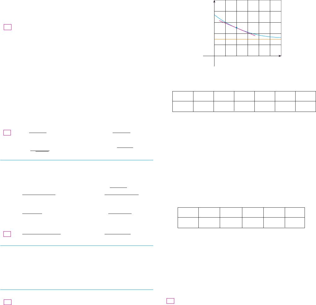
EXAMPLE 7 Let be the US national debt at time t. The table in the margin gives
approximate values of this function by providing end of year estimates, in billions of
dollars, from 1980 to 2000. Interpret and estimate the value of .
SOLUTION The derivative means the rate of change of D with respect to t when
, that is, the rate of increase of the national debt in 1990.
According to Equation 5,
So we compute and tabulate values of the difference quotient (the average rates of
change) as shown in the table at the left. From this table we see that lies some-
where between 257.48 and 348.14 billion dollars per year. [Here we are making the
reasonable assumption that the debt didn’t fluctuate wildly between 1980 and 2000.] We
estimate that the rate of increase of the national debt of the United States in 1990 was
the average of these two numbers, namely
Another method would be to plot the debt function and estimate the slope of the tan-
gent line when .
M
In Examples 3, 6, and 7 we saw three specific examples of rates of change: the veloci-
ty of an object is the rate of change of displacement with respect to time; marginal cost is
the rate of change of production cost with respect to the number of items produced; the
rate of change of the debt with respect to time is of interest in economics. Here is a small
sample of other rates of change: In physics, the rate of change of work with respect to time
is called power. Chemists who study a chemical reaction are interested in the rate of
change in the concentration of a reactant with respect to time (called the rate of reaction).
A biologist is interested in the rate of change of the population of a colony of bacteria with
respect to time. In fact, the computation of rates of change is important in all of the natu-
ral sciences, in engineering, and even in the social sciences. Further examples will be given
in Section 3.7.
All these rates of change are derivatives and can therefore be interpreted as slopes of
tangents. This gives added significance to the solution of the tangent problem. Whenever
we solve a problem involving tangent lines, we are not just solving a problem in geome-
try. We are also implicitly solving a great variety of problems involving rates of change in
science and engineering.
t ! 1990
D%!1990" % 303 billion dollars per year
D%!1990"
D%!1990" ! lim
t l1990
D!t" ! D!1990"
t ! 1990
t ! 1990
D%!1990"
D%!1990"
D!t"
V
SECTION 3.1 DERIVATIVES AND RATES OF CHANGE
|| ||
119
t
1980 930.2
1985 1945.9
1990 3233.3
1995 4974.0
2000 5674.2
D!t"
t
1980 230.31
1985 257.48
1995 348.14
2000 244.09
D!t" ! D!1990"
t ! 1990
N A NOTE ON UNITS
The units for the average rate of change
are the units for divided by the units for ,
namely, billions of dollars per year. The instan-
taneous rate of change is the limit of the aver-
age rates of change, so it is measured in the
same units: billions of dollars per year.
&t&D
&D#&t
What do you notice about the curve as you zoom in toward
the origin?
3. (a) Find the slope of the tangent line to the parabola
at the point
(i) using Definition 1 (ii) using Equation 2
(b) Find an equation of the tangent line in part (a).
!1, 3"y ! 4x ! x
2
1. A curve has equation .
(a) Write an expression for the slope of the secant line
through the points and .
(b) Write an expression for the slope of the tangent line at P.
;
2. Graph the curve in the viewing rectangles
by , by , and by .&!0.5, 0.5'&!0.5, 0.5'&!1, 1'&!1, 1'&!2, 2'
&!2, 2'y ! sin x
Q!x, f !x""P!3, f !3""
y ! f !x"
E X E R C I S E S
3.1
(b) At what time is the distance between the runners the
greatest?
(c) At what time do they have the same velocity?
If a ball is thrown into the air with a velocity of 40 ft#s, its
height (in feet) after seconds is given by .
Find the velocity when .
14. If a rock is thrown upward on the planet Mars with a velocity
of , its height (in meters) after seconds is given by
.
(a) Find the velocity of the rock after one second.
(b) Find the velocity of the rock when .
(c) When will the rock hit the surface?
(d) With what velocity will the rock hit the surface?
15. The displacement (in meters) of a particle moving in a
straight line is given by the equation of motion ,
where is measured in seconds. Find the velocity of the
particle at times , and .
16. The displacement (in meters) of a particle moving in a
straight line is given by , where is mea-
sured in seconds.
(a) Find the average velocity over each time interval:
(i) (ii)
(iii) (iv)
(b) Find the instantaneous velocity when .
(c) Draw the graph of as a function of and draw the secant
lines whose slopes are the average velocities in part (a)
and the tangent line whose slope is the instantaneous
velocity in part (b).
For the function t whose graph is given, arrange the follow-
ing numbers in increasing order and explain your reasoning:
(a) Find an equation of the tangent line to the graph of
at if and .
(b) If the tangent line to at (4, 3) passes through the
point (0, 2), find and .
Sketch the graph of a function for which ,
, and .
20. Sketch the graph of a function for which
, , and .t%!2" ! 1t%!1" ! 3t%!!1" ! !1
t!0" ! t%!0" ! 0,t
f %!2" ! !1f %!1" ! 0f %!0" ! 3,
f !0" ! 0f
19.
f %!4"f !4"
y ! f !x"
t%!5" ! 4t!5" ! !3x ! 5y ! t!x"
18.
y=©
1 3 4_1
0
x
2
y
0 t%!!2" t%!0" t%!2" t%!4"
17.
ts
t ! 4
&4, 4.5'&4, 5'
&3.5, 4'&3, 4'
ts ! t
2
! 8t " 18
t ! 3t ! a, t ! 1, t ! 2
t
s ! 1#t
2
t ! a
H ! 10t ! 1.86t
2
t10 m#s
t ! 2
y ! 40t ! 16t
2
t
13.
;
(c) Graph the parabola and the tangent line. As a check on
your work, zoom in toward the point until the
parabola and the tangent line are indistinguishable.
4. (a) Find the slope of the tangent line to the curve
at the point
(i) using Definition 1 (ii) using Equation 2
(b) Find an equation of the tangent line in part (a).
;
(c) Graph the curve and the tangent line in successively
smaller viewing rectangles centered at until the
curve and the line appear to coincide.
5– 8 Find an equation of the tangent line to the curve at the
given point.
6.
8.
(a) Find the slope of the tangent to the curve
at the point where .
(b) Find equations of the tangent lines at the points
and .
;
(c) Graph the curve and both tangents on a common screen.
10. (a) Find the slope of the tangent to the curve at
the point where .
(b) Find equations of the tangent lines at the points
and .
;
(c) Graph the curve and both tangents on a common screen.
11. (a) A particle starts by moving to the right along a horizontal
line; the graph of its position function is shown. When is
the particle moving to the right? Moving to the left?
Standing still?
(b) Draw a graph of the velocity function.
12. Shown are graphs of the position functions of two runners,
and , who run a 100-m race and finish in a tie.
(a) Describe and compare how the runners run the race.
s (meters)
0
4 8 12
80
40
t (seconds)
A
B
B
A
s (meters)
0
2 4 6
4
2
t (seconds)
(
4,
1
2
)
!1, 1"
x ! a
y ! 1#
s
x
!2, 3"
!1, 5"
x ! ay ! 3 " 4x
2
! 2x
3
9.
!0, 0"y !
2x
!x " 1"
2
,
(
1, 1"y !
s
x
,
7.
!!1, 3"y ! 2x
3
! 5x,!3, 2"y !
x ! 1
x ! 2
,
5.
!1, 0"
!1, 0"
y ! x ! x
3
!1, 3"
120
|| ||
CHAPTER 3 DERIVATIVES
temperature. By measuring the slope of the tangent, estimate
the rate of change of the temperature after an hour.
41. The table shows the estimated percentage of the population
of Europe that use cell phones. (Midyear estimates are given.)
(a) Find the average rate of cell phone growth
(i) from 2000 to 2002 (ii) from 2000 to 2001
(iii) from 1999 to 2000
In each case, include the units.
(b) Estimate the instantaneous rate of growth in 2000 by
taking the average of two average rates of change. What
are its units?
(c) Estimate the instantaneous rate of growth in 2000 by mea-
suring the slope of a tangent.
42. The number of locations of a popular coffeehouse chain is
given in the table. (The numbers of locations as of June 30
are given.)
(a) Find the average rate of growth
(i) from 2000 to 2002 (ii) from 2000 to 2001
(iii) from 1999 to 2000
In each case, include the units.
(b) Estimate the instantaneous rate of growth in 2000 by
taking the average of two average rates of change. What
are its units?
(c) Estimate the instantaneous rate of growth in 2000 by mea-
suring the slope of a tangent.
The cost (in dollars) of producing units of a certain com-
modity is .
(a) Find the average rate of change of with respect to
when the production level is changed
(i) from to
(ii) from to
(b) Find the instantaneous rate of change of with respect to
when . (This is called the marginal cost.
Its significance will be explained in Section 3.7.)
x ! 100x
C
x ! 101x ! 100
x ! 105x ! 100
xC
C!x" ! 5000 " 10x " 0.05x
2
x
43.
N
P
P
T
(°F)
0
30 60 90 120 150
100
200
t (min)
21. If , find and use it to find an equation
of the tangent line to the parabola at the
point .
22. If , find and use it to find an equation of
the tangent line to the curve at the point .
(a) If , find and use it to find an
equation of the tangent line to the curve
at the point .
;
(b) Illustrate part (a) by graphing the curve and the tangent
line on the same screen.
24. (a) If , find and use it to find equa-
tions of the tangent lines to the curve at
the points and .
;
(b) Illustrate part (a) by graphing the curve and the tangent
lines on the same screen.
25–30 Find .
25. 26.
28.
29. 30.
31–36 Each limit represents the derivative of some function at
some number . State such an and in each case.
31. 32.
33. 34.
36.
37–38 A particle moves along a straight line with equation of
motion , where is measured in meters and in seconds.
Find the velocity and the speed when .
37. 38.
A warm can of soda is placed in a cold refrigerator. Sketch
the graph of the temperature of the soda as a function of time.
Is the initial rate of change of temperature greater or less than
the rate of change after an hour?
40. A roast turkey is taken from an oven when its temperature
has reached 185°F and is placed on a table in a room where
the temperature is 75°F. The graph shows how the tempera-
ture of the turkey decreases and eventually approaches room
39.
f !t" ! t
!1
! tf !t" ! 100 " 50t ! 4.9t
2
t ! 5
tss ! f !t"
lim
t
l
1
t
4
" t ! 2
t ! 1
lim
h
l
0
cos!
'
" h" " 1
h
35.
lim
x
l
'
#4
tan x ! 1
x !
'
#4
lim
x
l
5
2
x
! 32
x ! 5
lim
h
l
0
s
4
16 " h
! 2
h
lim
h
l
0
!1 " h"
10
! 1
h
afa
f
f !x" !
s
3x " 1
f !x" !
1
s
x " 2
f !x" !
x
2
" 1
x ! 2
f !t" !
2t " 1
t " 3
27.
f !t" ! t
4
! 5tf !x" ! 3 ! 2x " 4x
2
f %!a"
!3, 9"!2, 8"
y ! 4x
2
! x
3
G%!a"G!x" ! 4x
2
! x
3
!2, 2"
y ! 5x#!1 " x
2
"
F%!2"F!x" ! 5x#!1 " x
2
"
23.
!0, 1"y ! 1 ! x
3
t%!0"t!x" ! 1 ! x
3
!2, 2"
y ! 3x
2
! 5x
f %!2"f !x" ! 3x
2
! 5x
SECTION 3.1 DERIVATIVES AND RATES OF CHANGE
|| ||
121
Year 1998 1999 2000 2001 2002 2003
P 28 39 55 68 77 83
Year 1998 1999 2000 2001 2002
N 1886 2135 3501 4709 5886