Simmons C.H., Dennis E.M. Manual of Engineering Drawing
Подождите немного. Документ загружается.

80 Manual of Engineering Drawing
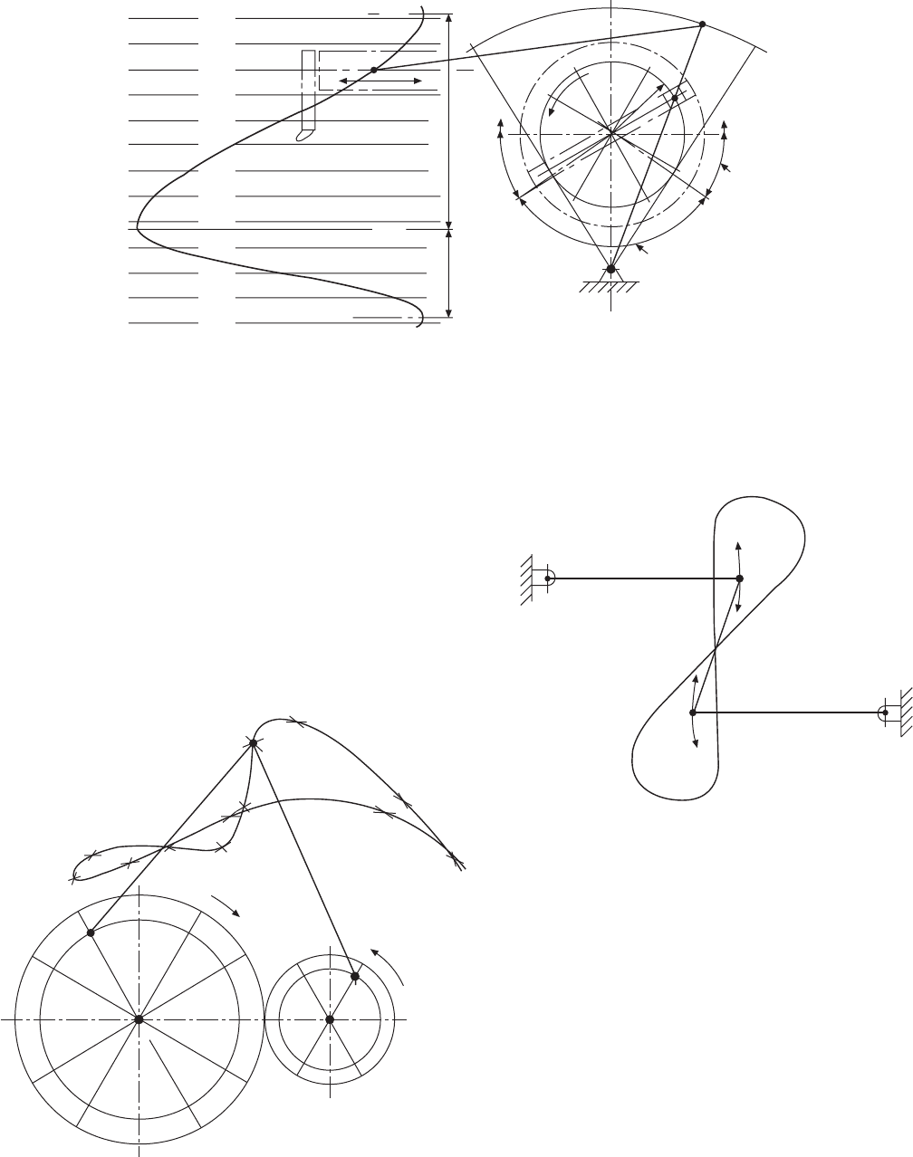
In Fig. 10.21 the radius OB has been increased,
with the effect of increasing the stroke of point D.
Note also that the return stroke in this condition is
quicker than before.
The outlines of two gears are shown in Fig. 10.22,
where the pitch circle of the larger gear is twice the
pitch circle of the smaller gear. As a result, the smaller
gear rotates twice while the larger gear rotates once.
The mechanism has been drawn in twelve positions to
plot the path of the pivot point C, where links BC and
CA are connected. A trammel method cannot be applied
successfully in this type of problem.
Figure 10.23 gives an example of Watt’s straight-
line motion. Two levers AX and BY are connected by
a link AB, and the plotted curve is the locus of the
Fig. 10.21
240
270
300
330
0
30
60
90
120
150
180
210
240
Displacement diagram
124
D
236
Forward
Return
C
0
90
R
B
270
Ο
180
A
Return stroke
Forward
stroke
4
3
5
2
C
1
12
6
1110
7
9
8
B
1
2
3
4
5
6
7
8
9
10
11
12
2
8
A
7
12 6
3 9
Q
10
4
11
5
P
X
A
P
B
Y
Fig. 10.22
Fig. 10.23 Watt’s straight line motion
Loci applications 81
mid-point P. The levers in this instance oscillate in
circular arcs. This mechanism was used in engines
designed by James Watt, the famous engineer.
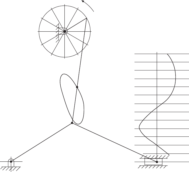
A toggle action is illustrated in Fig. 10.24, where a
crank rotates anticlockwise. Links AC, CD and CE
are pivoted at C. D is a fixed pivot point, and E slides
along the horizontal axis. The displacement diagram
has been plotted as previously described, but note that,
as the mechanism at E slides to the right, it is virtually
stationary between points 9, 10 and 11.
The locus of any point B is also shown.
Fig. 10.24
A
5
4
3
2
1
12
11
10
9
8
7
6
B
C
D
E
1
12
11
10
9
8
7
6
5
4
3
2
1
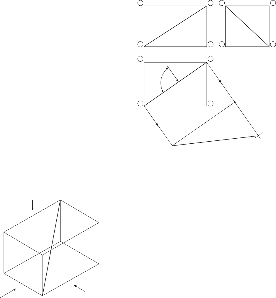
An isometric view of a rectangular block is shown in
Fig. 11.1. The corners of the block are used to position
a line DF in space. Three orthographic views in first-
angle projection are given in Fig. 11.2, and it will be
apparent that the projected length of the line DF in
each of the views will be equal in length to the diagonals
across each of the rectangular faces. A cross check
with the isometric view will clearly show that the true
length of line DF must be greater than any of the
diagonals in the three orthographic views. The corners
nearest to the viewing position are shown as ABCD
etc.; the corners on the remote side are indicated in
rings. To find the true length of DF, an auxiliary
projection must be drawn, and the viewing position
must be square with line DF. The first auxiliary
projection in Fig. 11.2 gives the true length required,
which forms part of the right-angled triangle DFG.
Note that auxiliary views are drawn on planes other
than the principal projection planes. A plan is projected
from an elevation and an elevation from a plan. Since
this is the first auxiliary view projected, and from a
true plan, it is known as a first auxiliary elevation.
Other auxiliary views could be projected from this
auxiliary elevation if so required.
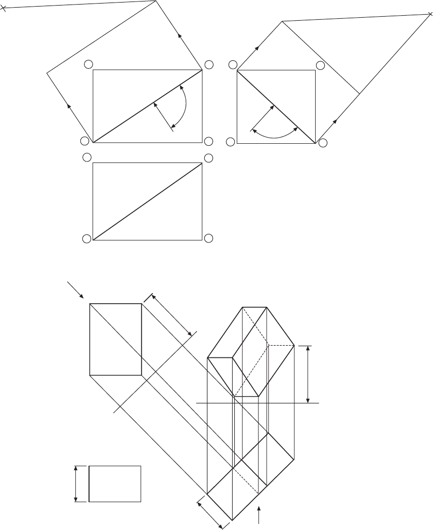
The true length of DF could also have been obtained
by projection from the front or end elevations by viewing
at 90° to the line, and Fig. 11.3 shows these two
alternatives. The first auxiliary plan from the front
elevation gives triangle FDH, and the first auxiliary
plan from the end elevation gives triangle FCD, both
right-angled triangles.
Figure 11.4 shows the front elevation and plan view
of a box. A first auxiliary plan is drawn in the direction
of arrow X. Now PQ is an imaginary datum plane at
right angles to the direction of viewing; the
perpendicular distance from corner A to the plane is
shown as dimension 1. When the first auxiliary plan
view is drawn, the box is in effect turned through 90°
in the direction of arrow X, and the corner A will be
situated above the plane at a perpendicular distance
equal to dimension 1. The auxiliary plan view is a true
view on the tilted box. If a view is now taken in the
direction of arrow Y, the tilted box will be turned through
90° in the direction of the arrow, and dimension 1 to
the corner will lie parallel with the plane of the paper.
The other seven corners of the box are projected as
indicated, and are positioned by the dimensions to the
plane PQ in the front elevation. A match-box can be
used here as a model to appreciate the position in
space for each projection.
Chapter 11
True lengths and auxiliary views
Plan
F
B
E
H
A
G
C
D
End
elevation
Front
elevation
Fig. 11.1
Fig. 11.2
E
F
F
B
H
H
GG C
G
C
D
Plan
Front elevation End elevation
True length
First auxiliary elevation
D
F
G
B
A
90°
E
F
DCHD
AB
E
A
True lengths and auxiliary views 83
The same box has been redrawn in Fig. 11.5, but
the first auxiliary elevation has been taken from the
plan view in a manner similar to that described in the
previous example. The second auxiliary plan projected
in line with arrow Y requires dimensions from plane
P
1
Q
1
, which are taken as before from plane PQ. Again,
check the projections shown with a match-box. All of
the following examples use the principles demonstrated
in these two problems.
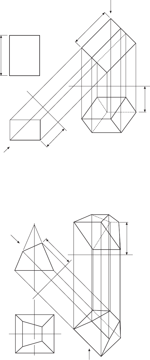
Part of a square pyramid is shown in Fig. 11.6; the
constructions for the eight corners in both auxiliary
views are identical with those described for the box in
Fig. 11.4.
Auxiliary projections from a cylinder are shown in
Fig. 11.7; note that chordal widths in the first auxiliary
plan are taken from the true plan. Each of twelve points
around the circle is plotted in this way and then projected
up to the auxiliary elevation. Distances from plane PQ
D
F
H
E
A
F
B
F
E
90°
B
A
F
D
C
C
D
90°
G
H
G
C
G
F
H
D
H
E
D
A
C
B
Fig. 11.3
X
A
I
Q
P
P1 Q1
A
Second auxiliary
elevation
1
2
2
Y
A
First auxiliary
plan
Fig. 11.4
84 Manual of Engineering Drawing
2
2
Y
A
First auxiliary
elevation
P1
Q1
1
Second
auxiliary plan
A
Q
P
1
A
X
Fig. 11.5
Fig. 11.6
X
I
P
Q
P1 Q1
1
Second auxiliary
elevation
Y
First auxiliary
plan
True lengths and auxiliary views 85
Second
auxiliary
elevation
A
1
X
P1
Q1
Q
A
P
1
2
2
A
Y
First
auxiliary plan
Fig. 11.7
True
shape
A
P
P2
P1
Q
F
A
2
Q1
1
G
1
A
3
2
A
4
Q2
P3
P4
Q3
3
3
A
Q4
A
True
shape
H
Fig. 11.8
are used from plane P
1
Q
1
. Auxiliary projections of
any irregular curve can be made by plotting the positions
of a succession of points from the true view and rejoining
them with a curve in the auxiliary view.
Figure 11.8 shows a front elevation and plan view
of a thin lamina in the shape of the letter L. The lamina
lies inclined above the datum plane PQ, and the front
elevation appears as a straight line. The true shape is
projected above as a first auxiliary view. From the
given plan view, an auxiliary elevation has been
projected in line with the arrow F, and the positions of
the corners above the datum plane P
1
Q
1
will be the
same as those above the original plane PQ. A typical
dimension to the corner A has been added as dimension
1. To assist in comprehension, the true shape given
could be cut from a piece of paper and positioned
above the book to appreciate how the lamina is situated
in space; it will then be seen that the height above the
book of corner A will be dimension 2.
Now a view in the direction of arrow G parallel
with the surface of the book will give the lamina shown
projected above datum P
2
Q
2
. The object of this exercise
is to show that if only two auxiliary projections are
given in isolation, it is possible to draw projections to
find the true shape of the component and also get the
component back, parallel to the plane of the paper.
The view in direction of arrow H has been drawn and
taken at 90° to the bottom edge containing corner A;
the resulting view is the straight line of true length
positioned below the datum plane P
3
Q
3
. The lamina is
situated in this view in the perpendicular position above
4
86 Manual of Engineering Drawing
the paper, with the lower edge parallel to the paper
and at a distance equal to dimension 4 from the surface.
View J is now drawn square to this projected view and
positioned above the datum P
4
Q
4
to give the true shape
of the given lamina.
In Fig. 11.9, a lamina has been made from the
polygon ACBD in the development and bent along the
axis AB; again, a piece of paper cut to this shape and
bent to the angle φ may be of some assistance. The
given front elevation and plan position the bent lamina
in space, and this exercise is given here since every
line used to form the lamina in these two views is not
a true length. It will be seen that, if a view is now
drawn in the direction of arrow X, which is at right
angles to the bend line AB, the resulting projection
will give the true length of AB, and this line will also
lie parallel with the plane of the paper. By looking
along the fold in the direction of arrow Y, the two
corners A and B will appear coincident; also, AD and
BC will appear as the true lengths of the altitudes DE
and FC. The development can now be drawn, since the
positions of points E and F are known along the true
length of AB. The lengths of the sides AD, DB, BC
and AC are obtained from the pattern development.
Fig. 11.9
C
B
A
D
1
Q
P
B
C
X
D
A
2
P1
Q1
D
1
P2
Q2
2
A
B
φ
C
D
F
B
E
D
Y
A
C
B
Development
C
A
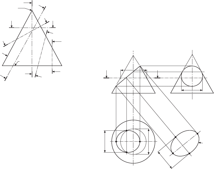
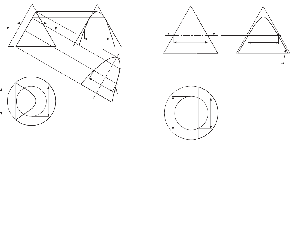
Consider a right circular cone, i.e. a cone whose base
is a circle and whose apex is above the centre of the
base (Fig. 12.1). The true face of a section through the
apex of the cone will be a triangle.
2 Project points A and B onto this line and onto the
centre lines of the plan and end elevation.
3 Take any horizontal section XX between A and B
and draw a circle in the plan view of diameter D.
4 Project the line of section plane XX onto the end
elevation.
5 Project the point of intersection of line AB and
plane XX onto the plan view.
6 Mark the chord-width W on the plan, in the auxiliary
view and the end elevation. These points in the
auxiliary view form part of the ellipse.
7 Repeat with further horizontal sections between A
and B, to complete the views as shown.
Chapter 12
Conic sections and interpenetration
of solids
C
F
A
B
B
F
Generator
Apex
D
E
E
D
A
C
Fig. 12.1 Conic sections: section AA – triangle; section BB – circle;
section CC – parabola; section DD – hyperbola; section EE – rect-
angular hyperbola; section FF – ellipse
The true face of a section drawn parallel to the base
will be a circle.
The true face of any other section which passes
through two opposite generators will be an ellipse.
The true face of a section drawn parallel to the
generator will be a parabola.
If a plane cuts the cone through the generator and
the base on the same side of the cone axis, then a view
on the true face of the section will be a hyperbola. The
special case of a section at right-angles to the base
gives a rectangular hyperbola.
To draw an ellipse from
part of a cone
Figure 12.2 shows the method of drawing the ellipse,
which is a true view on the surface marked AB of the
frustum of the given cone.
1 Draw a centre line parallel to line AB as part of an
auxiliary view.
X
A
φ
D
B
X
W
A
B
B
Ellipse
L
c
A
W
φ
D
B
A
W
Fig. 12.2
To draw a parabola from
part of a cone
Figure 12.3 shows the method of drawing the parabola,
which is a true view on the line AB drawn parallel to
the sloping side of the cone.
88 Manual of Engineering Drawing
1 Draw a centre line parallel to line AB as part of an
auxiliary view.
2 Project point B to the circumference of the base in
the plan view, to give the points B
1
and B
2
. Mark
chord-width B
1
B
2
in the auxiliary view and in the
end elevation.
3 Project point A onto the other three views.
4 Take any horizontal section XX between A and B
and draw a circle in the plan view of diameter D.
5 Project the line of section plane XX onto the end
elevation.
6 Project the point of intersection of line AB and
plane XX to the plane view.
7 Mark the chord-width W on the plan, in the end
elevation and the auxiliary view. These points in
the auxiliary view form part of the parabola.
8 Repeat with further horizontal sections between A
and B, to complete the three views.
To draw a rectangular
hyperbola from part
of a cone
Figure 12.4 shows the method of drawing the hyperbola,
which is a true view on the line AB drawn parallel to
the vertical centre line of the cone.
1 Project point B to the circumference of the base in
the plan view, to give the points B
1
and B
2
.
2 Mark points B
1
and B
2
in the end elevation.
3 Project point A onto the end elevation. Point A
lies on the centre line in the plan view.
4 Take any horizontal section XX between A and B
and draw a circle of diameter D in the plan view.
5 Project the line of section XX onto the end elevation.
6 Mark the chord-width W in the plan, on the end
elevation. These points in the end elevation form
part of the hyperbola.
7 Repeat with further horizontal sections between A
and B, to complete the hyperbola.
The ellipse, parabola, and hyperbola are also the loci
of points which move in fixed ratios from a line (the
directrix) and a point (the focus). The ratio is known
as the eccentricity.
Eccentricity =
distance from focus
perpendicular distance from directrix
The eccentricity for the ellipse is less than one.
The eccentricity for the parabola is one.
The eccentricity for the hyperbola is greater than
one.
Figure 12.5 shows an ellipse of eccentricity 3/5, a
parabola of eccentricity 1, and a hyperbola of
eccentricity 5/3. The distances from the focus are all
radial, and the distances from the directrix are per-
pendicular, as shown by the illustration.
To assist in the construction of the ellipse in Fig.
12.5, the following method may be used to ensure that
the two dimensions from the focus and directrix are in
the same ratio. Draw triangle PA1 so that side A1 and
side P1 are in the ratio of 3 units to 5 units. Extend
both sides as shown. From any points B, C, D, etc.,
draw vertical lines to meet the horizontal at 2, 3, 4,
etc.; by similar triangles, vertical lines and their
corresponding horizontal lines will be in the same ratio.
A similar construction for the hyperbola is shown in
Fig. 12.6.
Commence the construction for the ellipse by drawing
a line parallel to the directrix at a perpendicular distance
of P3 (Fig. 12.6 (a)). Draw radius C3 from point F
1
to
X
B
B1
B2
W
A
φ
D
B1
W
B2
Parabola
A
B2
B1
W
A
X
A
φ
D
Fig. 12.3
X
φ
D
B
B1
X
A
A
W
Hyperbola
B2
B2
B1
φ
D
A
W
Fig. 12.4
Conic sections and interpenetration of solids 89
Repeat the procedure in each case to obtain the
required curves.
Interpenetration
Many objects are formed by a collection of geometrical
shapes such as cubes, cones, spheres, cylinders, prisms,
pyramids, etc., and where any two of these shapes
meet, some sort of curve of intersection or
interpenetration results. It is necessary to be able to
draw these curves to complete drawings in orthographic
projection or to draw patterns and developments.
The following drawings show some of the most
commonly found examples of interpenetration.
Basically, most curves are constructed by taking sections
through the intersecting shapes, and, to keep
construction lines to a minimum and hence avoid
confusion, only one or two sections have been taken
in arbitrary positions to show the principle involved;
further similar parallel sections are then required to
establish the line of the curve in its complete form.
Where centre lines are offset, hidden curves will not
be the same as curves directly facing the draughtsman,
but the draughting principle of taking sections in the
manner indicated on either side of the centre lines of
the shapes involved will certainly be the same.
If two cylinders, or a cone and a cylinder, or two
cones intersect each other at any angle, and the curved
surfaces of both solids enclose the same sphere, then
the outline of the intersection in each case will be an
ellipse. In the illustrations given in Fig. 12.7 the centre
Directrix
P3
Q 3
Rad S2
Rad C3
F1
F2
Ellipse
Parabola
Hyperbola
Distance from focus
3 units
5 units
Perpendicular distance
from directrix
12 3 4 5 6
(a)
A
B
C
D
E
F
P
Distance from focus
5 units
3 units
Perpendicular distance
from directrix
12 3 4 5
(b)
R
S
T
U
V
Q
Fig. 12.5
Fig. 12.6 (a) Ellipse construction (b) Hyperbola construction
intersect this line. The point of intersection lies on the
ellipse. Similarly, for the hyperbola (Fig. 12.6 (b))
draw a line parallel to the directrix at a perpendicular
distance of Q2. Draw radius S2, and the hyperbola
passes through the point of intersection. No scale is
required for the parabola, as the perpendicular distances
and the radii are the same magnitude.
A
B
O
A
B
O
A
B
O
A
B
O
A
B
O
A
B
O
Fig. 12.7