Principles of Finance with Excel (Основы финансов c Excel)
Подождите немного. Документ загружается.

PFE Chapter 28, Charts and graphs in Excel page 13
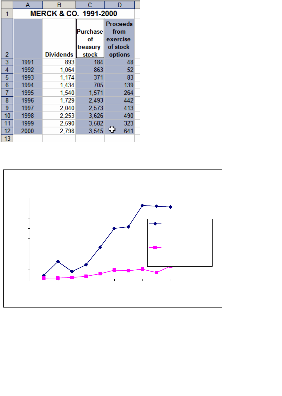
You can now follow the regular graphing procedure to create the following chart:
Merck Treasury Stock and Option Exercise
0
500
1,000
1,500
2,000
2,500
3,000
3,500
4,000
1990 1992 1994 1996 1998 2000 2002
Year
Purchase of
treasury stock
Proceeds from
exercise of stock
options
Fine-tuning—changing font size so that the axis labels fit
Look at the x-axis above: It goes from 1990 to 2002 even though the data only goes from
1991 – 2000. This often happens when Excel creates an x-axis for a graph. We’ve already
PFE Chapter 28, Charts and graphs in Excel page 14
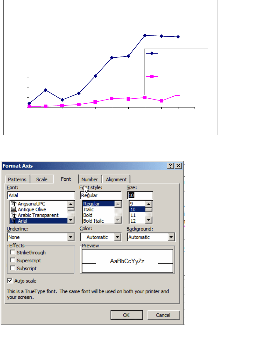
shown how to use the Format axis menu to change the axis. But this time when we do this, the
x-axis labels don’t fit properly:
Merck Treasury Stock and Option Exercise
0
500
1,000
1,500
2,000
2,500
3,000
3,500
4,000
1991 1992 1993 1994 1995 1996 1997 1998 1999 2000 2001
Year
Purchase of
treasury stock
Proceeds from
exercise of stock
options
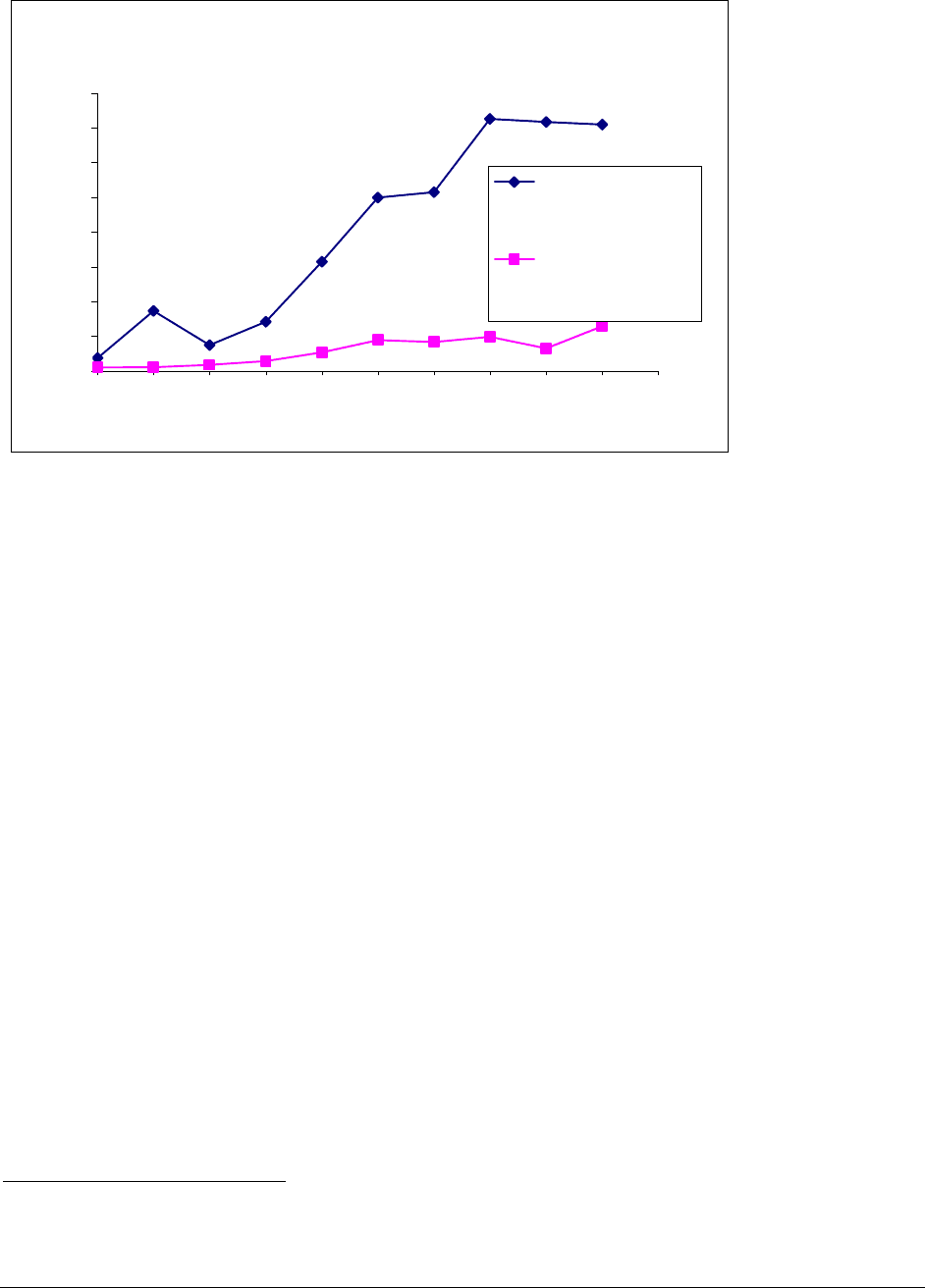
Go back into the dialog box and hit the Font tab to change the size of the x-axis font:
Now the graph looks fine:
PFE Chapter 28, Charts and graphs in Excel page 15
Merck Treasury Stock and Option Exercise
0
500
1,000
1,500
2,000
2,500
3,000
3,500
4,000
1991 1992 1993 1994 1995 1996 1997 1998 1999 2000 2001
Year
Purchase of
treasury stock
Proceeds from
exercise of stock
options
(There are other ways to accomplish this trick also—if you make the chart bigger, for
example.)
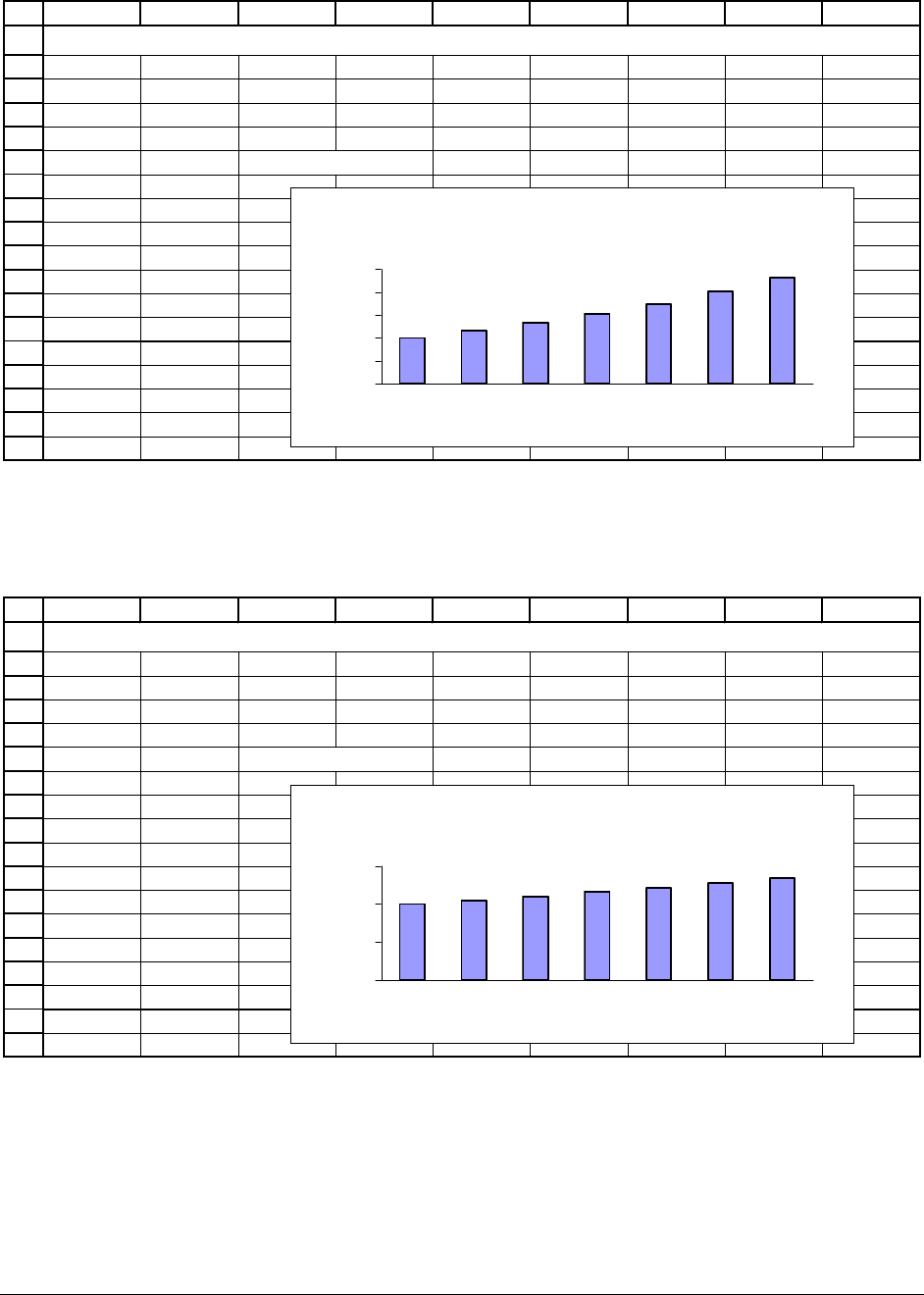
28.4. Graph titles that update
2
You want to have the graph title change when a parameter on the spreadsheet changes.
For example, in the next spreadsheet, you want the graph title to indicate the growth rate.
2
This section makes (largely self-explanatory) use of the Text function, which is discussed in Chapter 27.
PFE Chapter 28, Charts and graphs in Excel page 16
1
2
3
4
5
6
7
8
9
10
11
12
13
14
15
16
17
18
ABCDEFGH I
Growth 15%
Year Cash flow
1 100.00
2 115.00 <-- B6*(1+$B$3)
3 132.25
4 152.09
5 174.90
6 201.14
7 231.31
GRAPH TITLES THAT UPDATE AUTOMATICALLY
Cash Flow Graph When
Growth = 15.0%
0
50
100
150
200
250
1234567
Year
Cash flow
Once we have completed the necessary steps explained below, a change in the growth rate will
change both the graph and its title:
1
2
3
4
5
6
7
8
9
10
11
12
13
14
15
16
17
18
ABCDEFGH I
Growth 5%
Year Cash flow
1 100.00
2 105.00 <-- B6*(1+$B$3)
3 110.25
4 115.76
5 121.55
6 127.63
7 134.01
GRAPH TITLES THAT UPDATE AUTOMATICALLY
Cash Flow Graph When
Growth = 5.0%
0
50
100
150
1234567
Year
Cash flow
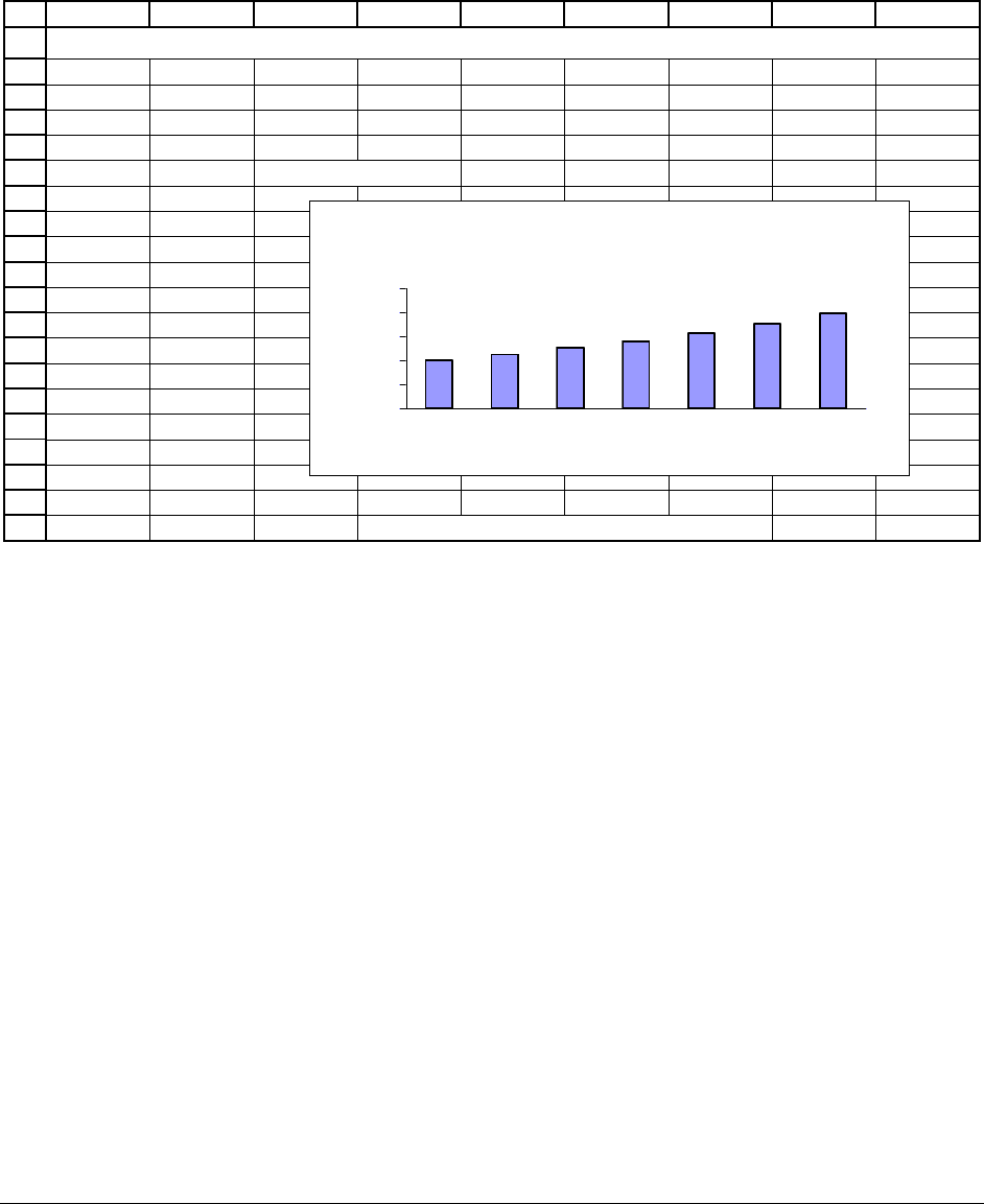
To make graph titles update automatically, carry out the following steps:
PFE Chapter 28, Charts and graphs in Excel page 17
• Create the graph you want in the format you want it. Give the graph a “proxy title.”
(It makes no difference what, you’re going to eliminate it soon.) At this stage your
graph might look like:
1
2
3
4
5
6
7
8
9
10
11
12
13
14
15
16
17
18
19
20
ABCDEFGH I
Growth 12%
Year Cash flow
1 100.00
2 112.00 <-- =B5*(1+$B$2)
3 125.44
4 140.49
5 157.35
6 176.23
7 197.38
Cash Flow Graph When Growth = 12.0%
GRAPH TITLES THAT UPDATE AUTOMATICALLY
asdf
0
50
100
150
200
250
1234567
Year
Cash flow
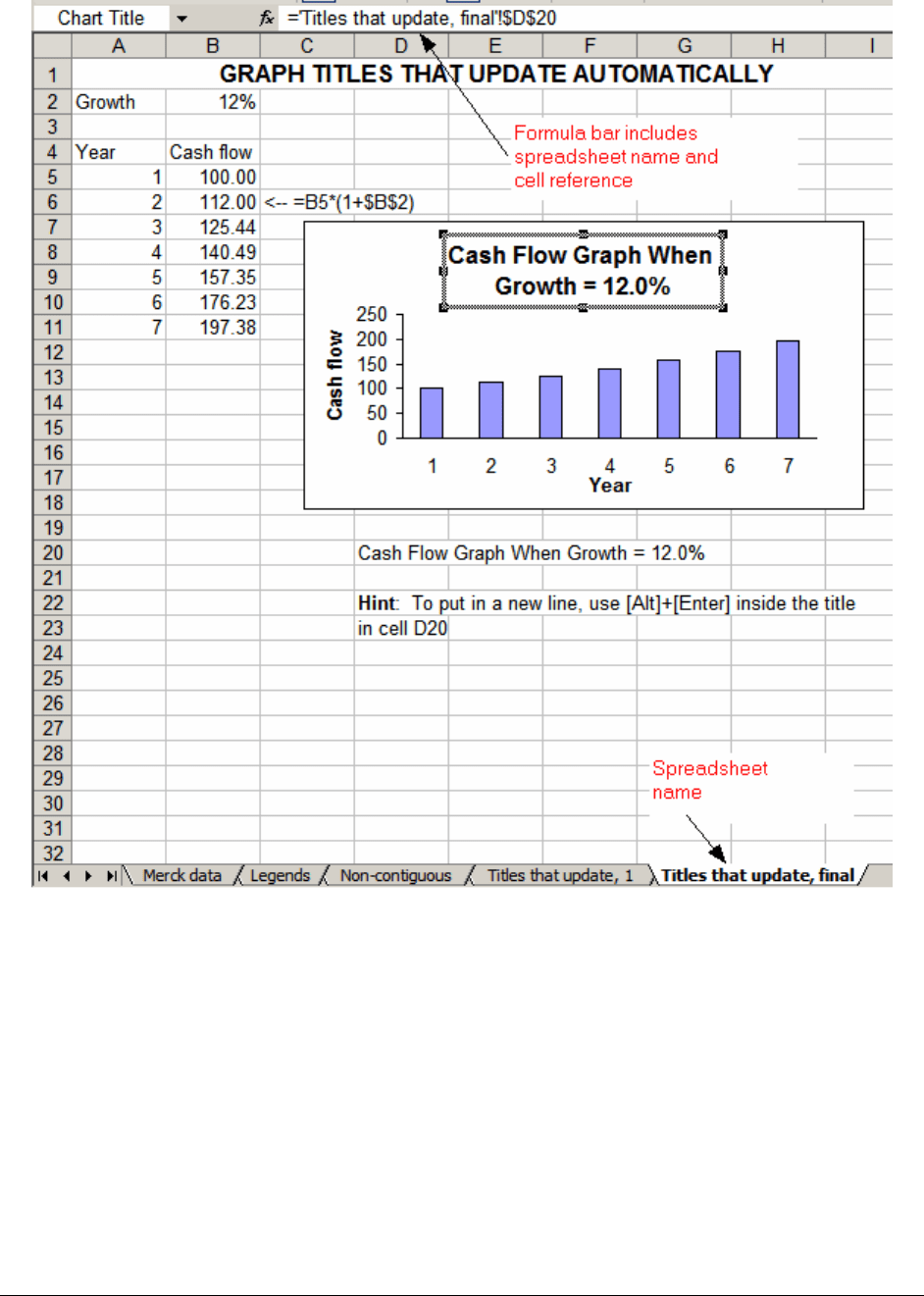
• Create the title you want in a cell. In the example above, cell D20 contains the formula:
="Cash Flow Graph when Growth = "&TEXT(B2,"0.0%").
• Click on the graph title to mark it, and then go to the formula bar and insert an equal sign
to indicate a formula. Then point at cell D20 with the formula and click [Enter]. In the
picture below, you see the chart title highlighted and in the formula bar “=Titles that
update!$D$20” indicating the title of the graph. Note that “Titles that update” is the
name of the spreadsheet.
PFE Chapter 28, Charts and graphs in Excel page 18
Summary
There’s lots more you can do with Excel charts, but we’ve covered the essentials. The
exercises to this chapter will show you some more variations.
PFE Chapter 28, Charts and graphs in Excel page 19
Exercises
Note: All the data for the exercises is on the CD-ROM which accompanies Principles of
Finance with Excel.
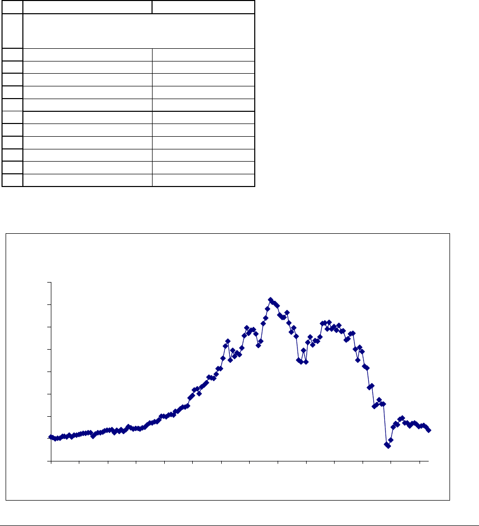
1. The CD gives the monthly prices for the Dutch grocery chain Ahold from April 1991 through
August 2004. Graph these prices.
1
2
3
4
5
6
7
8
9
10
11
12
AB
Date Stock price
8-Apr-91 5.32
1-May-91 5.23
3-Jun-91 4.94
1-Jul-91 5.03
1-Aug-91 5.09
3-Sep-91 5.43
1-Oct-91 5.40
1-Nov-91 5.37
2-Dec-91 5.68
2-Jan-92 5.39
PRICE OF AHOLD STOCK
April 1991 - August 2004
Your graph should look like this:
AHOLD STOCK PRICE
0.00
5.00
10.00
15.00
20.00
25.00
30.00
35.00
40.00
Apr-
91
Apr-
92
Apr-
93
Apr-
94
Apr-
95
Apr-
96
Apr-
97
Apr-
98
Apr-
99
Apr-
00
Apr-
01
Apr-
02
Apr-
03
Apr-
04
PFE Chapter 28, Charts and graphs in Excel page 20
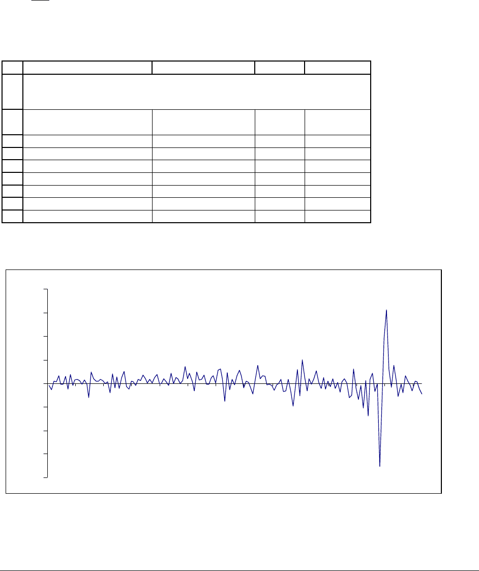
2. Using the data for Ahold from the previous exercise, determine the monthly stock returns and
graph them. The monthly return for a stock which has price P
t
in month t and price P
t-1
in month
t-1 is
1
1
t
t
P
P
−
− . (When you compute the returns, you’ll have “non-contiguous data,” so that you’ll
have to use the technique described in Section 28.3.)
1
2
3
4
5
6
7
8
9
ABCD
Date Stock price
Monthly
return
8-Apr-91 5.32
1-May-91 5.23 -1.69% <-- =B4/B3-1
3-Jun-91 4.94 -5.54% <-- =B5/B4-1
1-Jul-91 5.03 1.82% <-- =B6/B5-1
1-Aug-91 5.09 1.19%
3-Sep-91 5.43 6.68%
1-Oct-91 5.40 -0.55%
RETURNS ON AHOLD STOCK
April 1991 - August 2004
Your graph should look like this:
AHOLD STOCK RETURNS
-80%
-60%
-40%
-20%
0%
20%
40%
60%
80%
Apr-91 Apr-92 Apr-93 Apr-94 Apr-95 Apr-96 Apr-97 Apr-98 Apr-99 Apr-00 Apr-01 Apr-02 Apr-03 Apr-04
PFE Chapter 28, Charts and graphs in Excel page 21
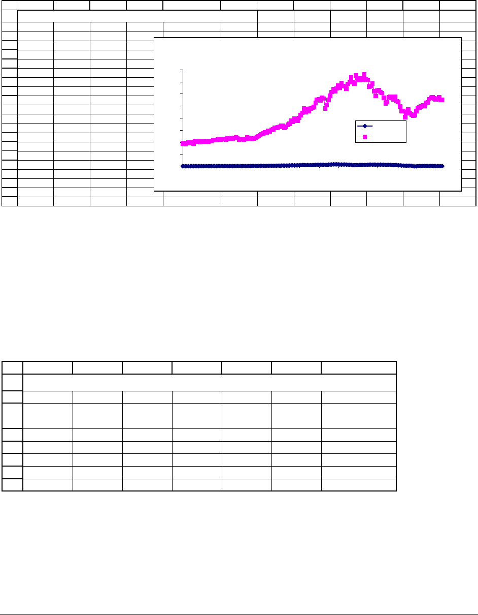
3. The CD with the book gives the prices for Ahold and for the S&P 500. Use this data to
produce the following graph (see note following the graph):
1
2
3
4
5
6
7
8
9
10
11
12
13
14
15
16
17
18
19
20
21
ABCD E FGH I J KL
AHOLD'S STOCK PRICE VERSUS THE S&P 500
Date Ahold
S&P 500
8-Apr-91 5.32 375.34
1-May-91 5.23 389.83
3-Jun-91 4.94 371.16
1-Jul-91 5.03 387.81
1-Aug-91 5.09 395.43
3-Sep-91 5.43 387.86
1-Oct-91 5.40 392.45
1-Nov-91 5.37 375.22
2-Dec-91 5.68 417.09
2-Jan-92 5.39 408.78
3-Feb-92 5.80 412.70
2-Mar-92 5.69 403.69
1-Apr-92 5.86 414.95
1-May-92 6.06 415.35
1-Jun-92 6.19 408.14
1-Jul-92 6.14 424.21
3-Aug-92 6.32 414.03
1-Sep-92 6.26 417.80
AHOLD PRICE vs S&P 500
0
200
400
600
800
1000
1200
1400
1600
Apr-91
Apr-92
Apr-93
Apr-94
Apr-95
Apr-96
Apr-97
Apr-98
Apr-99
Apr-00
Apr-01
Apr-02
Apr-03
Apr-04
Ahold
S&P 500
Note: This graph is obviously unsatisfactory—Ahold’s price is so much less than the S&P’s that
the Ahold price series appears to be zero. See the next exercise for one solution to this problem.
4. Transform the S&P and Ahold price data so that the beginning price of each is 100 and graph
these series:
1
2
3
4
5
6
7
8
ABCDEF G
AHOLD'S STOCK PRICE VERSUS THE S&P 500
Date Ahold
S&P 500
A
hold
adjusted
S&P
adjusted
8-Apr-91 5.32 375.34 100.00 100.00
1-May-91 5.23 389.83 98.31 103.86 <-- =F4*C5/C4
3-Jun-91 4.94 371.16 92.86 98.89 <-- =F5*C6/C5
1-Jul-91 5.03 387.81 94.55 103.32 <-- =F6*C7/C6
1-Aug-91 5.09 395.43 95.68 105.35
The final result should look like this:
PFE Chapter 28, Charts and graphs in Excel page 22
AHOLD PRICE vs S&P 500
0
100
200
300
400
500
600
700
800
Apr-91
Apr-92
Apr-93
Apr-94
Apr-95
Apr-96
Apr-97
Apr-98
Apr-99
Apr-00
Apr-01
Apr-02
Apr-03
Apr-04
Ahold
S&P 500
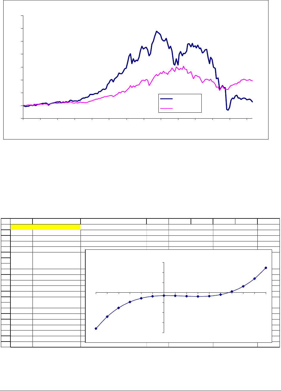
5. You have been asked to graph the function
32
216yax x x
=
−+−. The variable a can take on
a variety of values (in the example below, a = 0.4). Make a graph of this function with a title
that indicates the value of a, as illustrated below. (You may want to refer to Section 28.4.)
1
2
3
4
5
6
7
8
9
10
11
12
13
14
15
16
17
18
19
20
21
22
AB C DEFGHI
a0.4
x y=a*x^3-2*x^2+x-16
-6 -180.4 <-- =$B$1*A4^3-2*A4^2+A4-16
-5 -121.0
-4 -77.6
-3 -47.8
-2 -29.2
-1 -19.4
0 -16.0
1 -16.6
2 -18.8
3 -20.2
4 -18.4
5 -11.0
64.4
730.2
868.8
9 122.6
Graph of y=a*x^3-2*x^2+x-16 when a = 0.40
-200
-150
-100
-50
0
50
100
150
-6-5-4-3-2-10123456789
x