Nair S. Advanced Topics in Applied Mathematics: For Engineering and the Physical Sciences
Подождите немного. Документ загружается.


Laplace Transforms 199
To avoid confusion, we use s for the Laplace variable, instead of p,
and let
¯p(x,y, s) = L[p(x,y,t),t → s]. (4.156)
After taking the Laplace transform, we have
(∇
2
−k
2
s
2
) ¯p =0, ¯p(x,0,s) =
P
0
f (x)
s
, (4.157)
where k = 1/c. Next, we take the Fourier transform of the governing
equation and the boundary condition to get
∂
2
¯
P
∂y
2
−(ξ
2
+k
2
s
2
)
¯
P = 0,
¯
P(ξ ,0,s) =
P
0
F(ξ )
s
, (4.158)
where
¯
P = F[¯p,x →ξ ], F = F [f , x → ξ ]. (4.159)
Solution of this equation vanishing at infinity is
¯
P = Ae
−
√
ξ
2
+k
2
s
2
y
, (4.160)
where the square root has to be selected to have the real part of
ξ
2
+k
2
s
2
positive. This can be accomplished by introducing branch
cuts from iks to i∞ and from −iks to −i∞ in the complex ξ -plane.
Using the boundary condition, we find
A =P
0
F(ξ )/s. (4.161)
Thus,
¯
P(ξ ,y,s) =
P
0
F(ξ )
s
e
−
√
ξ
2
+k
2
s
2
y
. (4.162)
Recalling the Green’s functions, we express the solution in the
convolution form,
p(x,y,t) =P
0
∞
−∞
g(x −x
,y, t)f (x
)dx
, (4.163)
where
¯
G =FL[g(x, y,t)]=F [¯g(x,y, s)]=
1
√
2πs
e
−
√
ξ
2
+k
2
s
2
y
, (4.164)

200 Advanced Topics in Applied Mathematics
where we have inserted 1/
√
2π to avoid this factor in the anticipated
convolution integral for Fourier transforms.
A direct approach for inverting
¯
G requires a Fourier inversion inte-
gral and a Laplace inversion integral. Using the Cagniard-De Hoop
method, we can avoid actual integrations. The Fourier inverse is
written as
¯g(x, y,s) =
1
2π
∞
−∞
e
−
√
ξ
2
+k
2
s
2
y−iξ x
dξ
s
. (4.165)
A change of variable, ξ →sξ , gives
¯g(x, y,s) =
1
2π
∞
−∞
e
−s(
√
ξ
2
+k
2
y−iξ x)
dξ. (4.166)
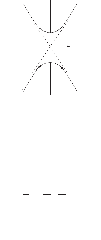
In Fig. 4.4, this integration is over the line, C. In the new ξ -plane
the branch points are at ±ik. We introduce new parameter t (which
will be later identified as time) to distort this line to , by defining
ξ
2
+k
2
y −iξ x = t,
(ξ
2
+k
2
)y
2
=(t +iξ x)
2
,
ξ
2
+
2itx
r
2
ξ +
k
2
y
2
−t
2
r
2
=0, r
2
=x
2
+y
2
. (4.167)
Solving for ξ,weget
ξ =±
√
t
2
−k
2
r
2
r
sinθ −i
t
r
cosθ , (4.168)
where
sinθ =y/r, cos θ = x/r. (4.169)
Let us distinguish the two roots as
ξ
+
=+
√
t
2
−k
2
r
2
r
sinθ −i
t
r
cosθ , (4.170)
ξ
−
=−
√
t
2
−k
2
r
2
r
sinθ −i
t
r
cosθ . (4.171)
Laplace Transforms 201
Re(ξ)
Im(ξ)
Γ
C
Figure 4.4. Distortion of the contour C to in the Cagniard-De Hoop method.
Note that as t varies from kr to ∞, the real part of ξ
+
varies from
0to∞, and the imaginary part varies from −k cosθ to −∞. This is
represented by the right half of the lower hyperbola in Fig. 4.4. For
large t, the slope of the hyperbola asymptotically approaches −cotθ .
The values of ξ from −∞ to 0 is covered by t going from ∞ to kr and
the asymptote for the left half of the lower hyperbola is cotθ.
The integral representation, Eq. (4.166), in terms of t is
¯g(x, y,s) =
1
2π
cr
∞
e
−st
dξ
−
dt
dt +
∞
cr
e
−st
dξ
+
dt
dt
=
1
2π
∞
cr
dξ
+
dt
−
dξ
−
dt
e
−st
dt. (4.172)
We recognize this expression as a Laplace transform with respect to
time, and the function g(x, y,t), which is the function we are looking
for, is the factor of e
−st
in the integrand. Then,
g(x, y,t) =
1
2π
dξ
+
dt
−
dξ
−
dt
h(t −kr), (4.173)

202 Advanced Topics in Applied Mathematics
where the Heaviside step function indicates a shift as our integrals start
from kr. Evaluation of the derivatives yields
dξ
+
dt
=
sinθ
r
t
√
t
2
−k
2
r
2
−i
cosθ
r
, (4.174)
dξ
+
dt
=−
sinθ
r
t
√
t
2
−k
2
r
2
−i
cosθ
r
, (4.175)
g(x, y,t) =
1
π
sinθ
r
t
√
t
2
−k
2
r
2
. (4.176)
The Green’s function we have found has the property that it is
the solution when P
0
f (x) = P
0
δ(x), a singular compressive force of
magnitude P
0
suddenly applied at the origin. The pressure for this
case is given by
p =
P
0
π
sinθ
r
t
√
t
2
−k
2
r
2
. (4.177)
When t →∞, we reach a steady-state solution,
p =
P
0
π
sinθ
r
, (4.178)
which is
p =−
P
0
π
Im(1/z), z =x +iy, (4.179)
and it satisfies the Laplace equation. In our original wave equation, the
right-hand term vanishes for steady-state solutions. For a concentrated
applied force of P
0
, we should have
P
0
= lim
r→0
π/2
0
2pr sin θ. (4.180)
As we can verify, our solution satisfies this equilibrium condition.
The Cagniard–De Hoop method has found numerous applications
in wave propagation problems in elastic media. The books by Fung
(1965)andEwing,JardetzkyandPress(1957)providefurthercitations
and solutions.

Laplace Transforms 203
4.10 SEQUENCES AND THE Z-TRANSFORM
Consider an infinite sequence of numbers
{a
n
}={a
0
,a
1
,..., a
n
,...}. (4.181)
We construct the so-called Z-transform of this sequence by multiplying
a
n
by z
n
and adding. Here, z is a complex number, and it is assumed that
the sequence is such that the sum converges for a suitable radius |z|.
Z{a
n
}=Z =
∞
0
a
n
z
n
. (4.182)
For example, the sequence
{1}={1, 1,...,1,...} (4.183)
gives
Z = 1 +z +z
2
+···=
1
1 −z
, (4.184)
provided |z|< 1. The sequence
{a
n
}={1, a,a
n
,...} (4.185)
has
Z = 1 +az +a
2
z
2
+···=
1
1 −az
. (4.186)
Our definition is slightly different from the commonly used definition –
we use z instead of z
−1
in our expansions.
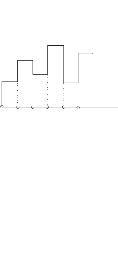
The connection between the Z-transform and the Laplace trans-
form will become clear if we convert the sequence into a discontinuous
function of time. Between t = 0andt = 1, the function has the value
of a
0
; between t = 1andt = 2, it has the value of a
1
, and so on.
This is shown in Fig. 4.5. Thus, the discontinuous function f (t) can
be written as
f (t) =a
0
[h(t) −h(t −1)]+a
1
[h(t −1) −h(t −2)]+···, (4.187)
204 Advanced Topics in Applied Mathematics
a
0
a
1
a
2
a
3
a
4
a
5
10354
t
f
2
Figure 4.5. Representation of a sequence as a discontinuous function.
where h is the Heaviside step function. The Laplace transform,
L[h(t −n) −h(t −n −1)]=
n+1
n
e
−pt
dt
=
1
p
e
−np
−e
−(n+1)p
=
e
−np
p
(1 −e
−p
).
(4.188)
Using this, we obtain the Laplace transform of our discontinuous
function,
¯
f =
1
p
(1 −e
−p
)
∞
0
a
n
e
−np
. (4.189)
A change of variable,
z =e
−p
, (4.190)
makes
¯
f =
z −1
Log z
Z, (4.191)

Laplace Transforms 205
where
Z =
∞
0
a
n
z
n
(4.192)
is the Z-transform. In choosing Log z, we have selected a branch along
the negative axis of Re (z).
Our elementary examples show that
Z
−1
1
1 −az
={a
n
}. (4.193)
In a more general case, the inverse Z-transform of a function F(z),
which is analytic within a circle around z =0, is the coefficient of z
n
in
the Taylor series expansion of F(z).
By differentiating Eq. (4.193) with respect to a,wefind
Z
−1
z
(1 −az)
2
={na
n−1
}. (4.194)
Similarly, by differentiating Eq. (4.186) with respect to z and
identifying the coefficient of z
n
,weget
Z
−1
a
(1 −az)
2
={(n +1)a
n+1
}. (4.195)
The relation between the Z-transform and the Laplace transform
makes it clear that the Laplace inversion integral can be used for
inverting more complicated Z-transforms.
4.10.1 Difference Equations
A sequence {u
n
} may be characterized by difference equations of the
form
u
n+1
=f (u
n
), (4.196)
where f is a given function. If f is a linear function, we have a linear
difference equation. As an initial condition, u
0
needs to be supplied
to begin the evaluation of u
1
, u
2
, etc. When the equation contains two

206 Advanced Topics in Applied Mathematics
consequent members, u
n+1
and u
n
, we have a first-order difference
equation. In addition to u
n+1
and u
n
, if it contains u
n+2
, we have a
second-order equation. Descretized versions of differential equations
(as in numerical analysis) yield difference equations.
4.10.2 First-Order Difference Equation
Consider the equation
u
n+1
=αu
n
+β. (4.197)
Here α and β are constants. If we denote the Z-transform of {u
n
}by Z,
Z = Z{u
n
}=
∞
0
u
n
z
n
. (4.198)
The Z-transform of the shifted sequence {u
n+1
} can be written as
Z{u
n+1
}=
∞
0
u
n+1
z
n
=z
−1
∞
0
u
n+1
z
n+1
=z
−1
∞
1
u
n
z
n
,
=z
−1
∞
0
u
n
z
n
−u
0
=z
−1
(Z −u
0
). (4.199)
With this, we can take the Z-transform of the first-order difference
equation, Eq. (4.197). This gives
z
−1
(Z −u
0
) =αZ +
β
1 −z
, (4.200)

Laplace Transforms 207
where we have used Z{1}=1/(1 −z). Solving for Z,
Z =
u
0
1 −αz
+
zβ
(1 −z)(1 −αz)
. (4.201)
Expanding the β-term in partial fractions yields
Z =
u
0
1 −αz
+
β
α −1
1
1 −αz
−
1
1 −z
. (4.202)
Inversion gives
u
n
=u
0
α
n
+β
α
n
−1
α −1
. (4.203)
4.10.3 Second-Order Difference Equation
The second-order homogeneous equation
u
n+2
−(b +c)u
n+1
+bcu
n
=0, (4.204)
with b and c being constants, may be transformed using
Z{u
n
}=Z, (4.205)
Z{u
n+1
}=z
−1
[Z −u
0
], Z{u
n+2
}=z
−2
[Z −u
0
−u
1
z], (4.206)
to obtain
Z −u
0
−u
1
z −(b +c)z[Z −u
0
]+bcz
2
Z = 0,
[1 −(b +c)z +bcz
2
]Z = u
0
+u
1
z −(b +c)u
0
z,
Z =
u
0
+u
1
z −(b +c)u
0
z
(1 −bz)(1 −cz)
=
u
0
b −c
b
1 −bz
−
c
1 −cz
+
u
1
−(b +c)u
0
b −c
1
1 −bz
−
1
1 −cz
=
u
1
−cu
0
b −c
1
1 −bz
−
u
1
−bu
0
b −c
1
1 −cz
. (4.207)

208 Advanced Topics in Applied Mathematics
After inversion, we get
u
n
=
u
1
−cu
0
b −c
b
n
−
u
1
−bu
0
b −c
c
n
. (4.208)
Note that this solution has two unknowns: u
0
and u
1
.
Example: Vibration of a String
The motion of a taut string occupying the spatial domain 0 < x <is
described by
Tu
=m¨u, (4.209)
where T is the string tension and m is the mass density per unit length.
Assuming harmonic motion in time, we assume
u(x,t) =v(x)e
it
, (4.210)
to reduce the equation to
v
=−m
2
v/T. (4.211)
Using
x/ →x, m
2
2
/T = ω
2
, (4.212)
we find
v
+ω
2
v = 0, 0 < x < 1. (4.213)
The well-known solution of this equation satisfying the boundary
conditions v(0) =v (1) =0is
v(x) =Asinωx, ω = nπ. (4.214)
Let us approximate the Eq. (4.213) using finite differences by dividing
the domain into N equal-length segments. If h is the length of a segment
Nh =1. (4.215)
The value of v at an arbitrary point x
n
= nh is denoted by v
n
and the
derivatives are approximated as
v
=
v
n+1
−v
n
h
, v
=
v
n+2
−2v
n+1
+v
n
h
2
. (4.216)