Mitchell Т. Machine learning
Подождите немного. Документ загружается.

which is wide enough to contain
95%
of the total probability under this distribu-
tion. This provides an interval surrounding
errorv(h)
into which
errors(h)
must
fall
95%
of the time. Equivalently, it provides the size of the interval surrounding
errordh)
into which
errorv(h)
must fall
95%
of the time.
For a given value of
N
how can we find the size of the interval that con-
tains
N%
of the probability mass? Unfortunately, for the Binomial distribution
this calculation can be quite tedious. Fortunately, however, an easily calculated
and very good approximation can be found in most cases, based on the fact that
for sufficiently large sample sizes the Binomial distribution can be closely ap-
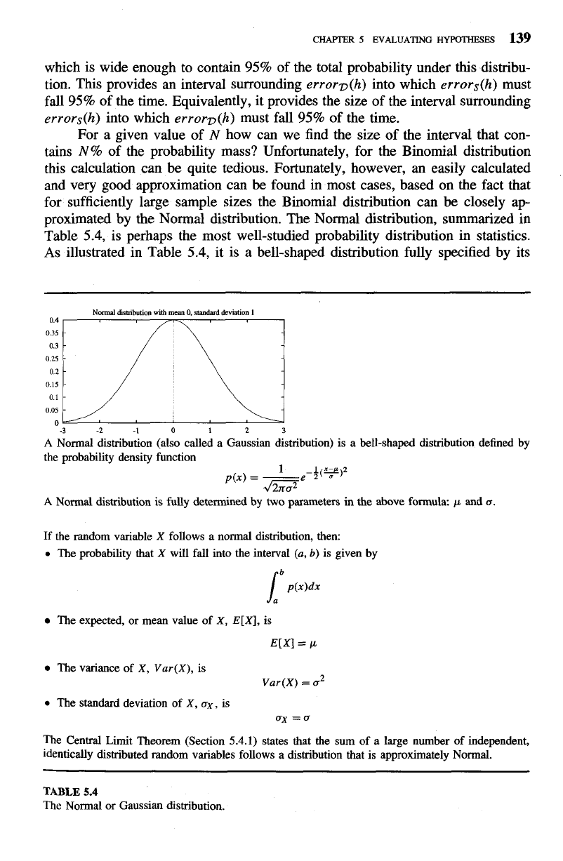
proximated by the Normal distribution. The Normal distribution, summarized in
Table
5.4,
is perhaps the most well-studied probability distribution in statistics.
As illustrated in Table
5.4,
it is a bell-shaped distribution fully specified by its
Normal
dismbution
with
mean
0.
standard
deviation
I
3
-2 -1
0
1
2
3
A
Normal distribution (also called a Gaussian distribution) is a bell-shaped distribution defined by
the probability density function
A
Normal distribution is fully determined by two parameters in the above formula:
p
and
a.
If
the random variable
X
follows a normal distribution, then:
0
The probability that
X
will fall into the interval
(a,
6)
is given by
The expected, or mean value of
X, E[X],
is
The variance of
X,
Var(X),
is
Var(X)
=
a2
0
The standard deviation of
X,
ax,
is
ax
=
a
The Central Limit Theorem (Section
5.4.1)
states that the sum of a large number of independent,
identically distributed random variables follows a distribution that is approximately Normal.
TABLE
5.4
The
Normal or Gaussian distribution.
mean
p
and standard deviation
a.
For large
n,
any Binomial distribution is very
closely approximated by a Normal distribution with the same mean and variance.
One reason that we prefer to work with the Normal distribution is that most
statistics references give tables specifying the size of the interval about the mean
that contains
N%
of the probability mass under the Normal distribution. This is
precisely the information needed to calculate our
N%
confidence interval. In fact,
Table 5.1 is such a table. The constant
ZN
given in Table 5.1 defines the width
of the smallest interval about the mean that includes
N%
of the total probability
mass under the bell-shaped Normal distribution. More precisely,
ZN
gives half the
width of the interval (i.e., the distance from the mean in either direction) measured
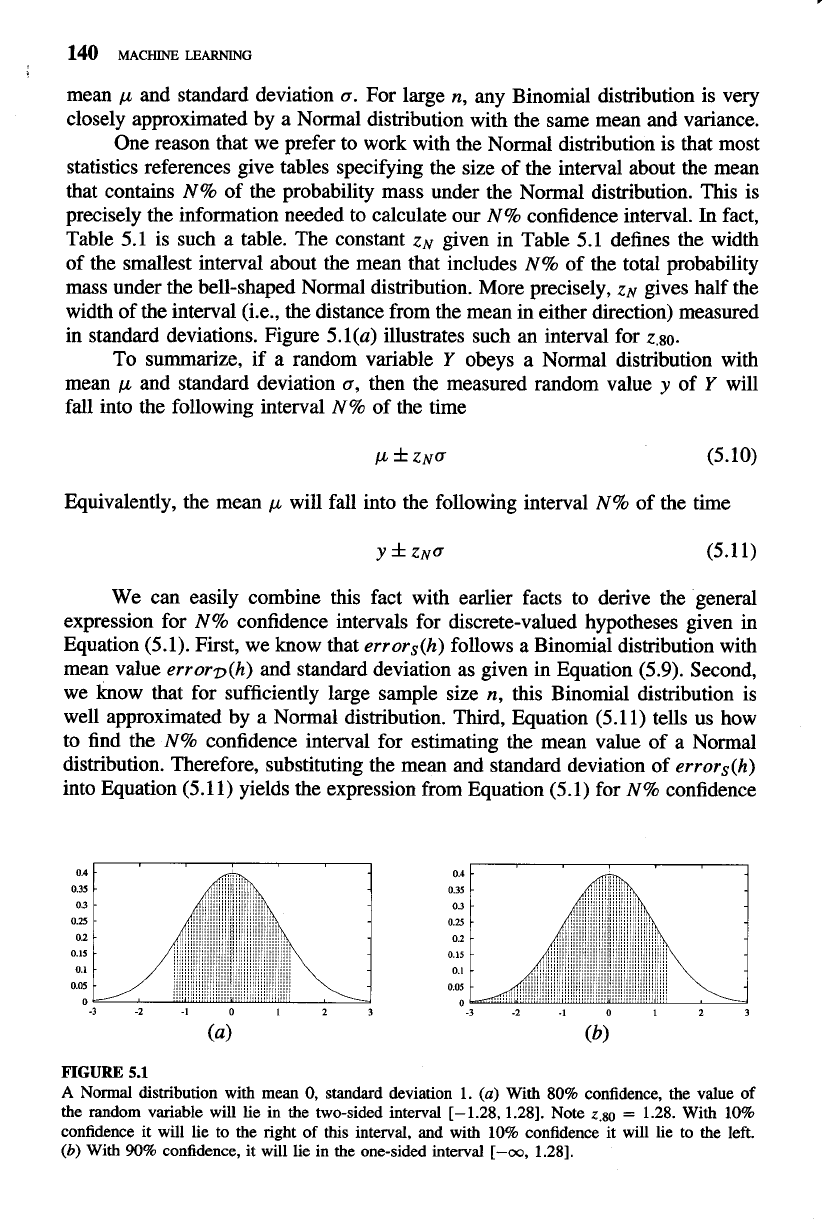
in standard deviations. Figure 5.l(a) illustrates such an interval for
z.80.
To summarize, if a random variable
Y
obeys a Normal distribution with
mean
p
and standard deviation a, then the measured random value
y
of
Y
will
fall into the following interval
N%
of the time
Equivalently, the mean
p
will fall into the following interval
N%
of the time
We can easily combine this fact with earlier facts to derive the general
expression for
N%
confidence intervals for discrete-valued hypotheses given in
Equation (5.1). First, we know that
errors(h)
follows a Binomial distribution with
mean value
error~(h)
and standard deviation as given in Equation (5.9). Second,
we know that for sufficiently large sample size
n,
this Binomial distribution is
well approximated by a Normal distribution. Third, Equation (5.1 1) tells us how
to find the
N%
confidence interval for estimating the mean value of a Normal
distribution. Therefore, substituting the mean and standard deviation of
errors(h)
into Equation (5.1 1) yields the expression from Equation (5.1) for
N%
confidence
FIGURE
5.1
A
Normal distribution with mean
0,
standard deviation
1.
(a)
With 80% confidence, the value of
the random variable will lie in the two-sided interval [-1.28,1.28]. Note
2.80
=
1.28. With 10%
confidence it will lie to the right of this interval, and with 10% confidence it will lie to the left.
(b)
With
90%
confidence, it will lie in the one-sided interval
[-oo,
1.281.
intervals for discrete-valued hypotheses
J
errors(h)(l
-
errors(h))
errors(h)
zt
ZN
n
Recall that two approximations were involved in deriving this expression, namely:
1.
in estimating the standard deviation
a
of errors(h), we have approximated
errorv(h) by errors(h) [i.e., in going from Equation (5.8) to (5.9)], and
2.
the Binomial distribution has been approximated by the Normal distribution.
The common rule of thumb in statistics is that these two approximations are very
good as long as n
2
30, or when np(1-
p)
2
5. For smaller values of n it is wise
to use a table giving exact values for the Binomial distribution.
5.3.6
Two-sided and One-sided Bounds
Notice that the above confidence interval is a two-sided bound; that is, it bounds
the estimated quantity from above and from below. In some cases, we will
be
interested only in a one-sided bound. For example, we might be interested in the
question "What is the probability that errorz,(h) is at most
U?'
This kind of one-
sided question is natural when we are only interested in bounding the maximum
error of h and do not mind if the true error is much smaller than estimated.
There is an easy modification to the above procedure for finding such one-
sided error bounds. It follows from the fact that the Normal distribution is syrnrnet-
ric about its mean. Because of this fact, any two-sided confidence interval based on
a
Normal distribution can be converted to a corresponding one-sided interval with
twice the confidence (see Figure 5.l(b)). That is, a 100(1- a)% confidence inter-
val with lower bound
L
and
upper bound
U
implies a 100(1- a/2)% confidence
interval with lower bound
L
and no upper bound. It also implies a 100(1 -a/2)%
confidence interval with upper bound
U
and no lower bound. Here
a
corresponds
to the probability that the correct value lies outside the stated interval. In other
words,
a
is the probability that the value will fall into the unshaded region in
Figure 5.l(a), and a/2 is the probability that it will fall into the unshaded region
in Figure
5.l(b).
To illustrate, consider again the example in which h commits r
=
12 errors
over a sample of n
=
40 independently drawn examples. As discussed above,
this leads to a (two-sided) 95% confidence interval of 0.30
f
0.14.
In
this case,
100(1
-
a)
=
95%, so
a!
=
0.05. Thus, we can apply the above rule to say with
100(1
-
a/2)
=
97.5% confidence that errorv(h) is at most 0.30
+
0.14
=
0.44,
making no assertion about the lower bound on errorv(h). Thus, we have a one-
sided error bound on
errorv(h) with double the confidence that we had in the
corresponding two-sided bound (see Exercise
5.3).
142
MACHINE
LEARNING
5.4 A GENERAL APPROACH FOR DERIVING CONFIDENCE
INTERVALS
The previous section described in detail how to derive confidence interval es-
timates for one particular case: estimating
errorv(h)
for a discrete-valued hy-
pothesis
h,
based on a sample of
n
independently drawn instances. The approach
described there illustrates a general approach followed in many estima6on prob-
lems.
In
particular, we can see this as a problem of estimating the mean (expected
value) of a population based on the mean of a randomly drawn sample of size
n.
The general process includes the following steps:
1.
Identify the underlying population parameter
p
to be estimated, for example,
errorv(h).
2.
Define the estimator
Y
(e.g.,
errors(h)).
It is desirable to choose a minimum-
variance, unbiased estimator.
3.
Determine the probability distribution
Vy
that governs the estimator Y, in-
cluding its mean and variance.
4.
Determine the
N%
confidence interval by finding thresholds
L
and
U
such
that
N%
of the mass in the probability distribution
Vy
falls between
L
and
U.
In later sections of this chapter we apply this general approach to sev-
eral other estimation problems common in machine learning. First, however, let
us discuss a fundamental result from estimation theory called the
Central Limit
Theorem.
5.4.1 Central Limit Theorem
One essential fact that simplifies attempts to derive confidence intervals is the
Central Limit Theorem. Consider again our general setting, in which we observe
the values of
n
independently drawn random variables
Yl
. . .
Yn
that obey the same
unknown underlying probability distribution (e.g.,
n
tosses of the same coin). Let
p
denote the mean of the unknown distribution governing each of the
Yi
and let
a
denote the standard deviation. We say that these variables
Yi
are
independent,
identically distributed
random variables, because they describe independent exper-
iments, each obeying the same underlying probability distribution.
In
an attempt
to estimate the mean
p
of the distribution governing the Yi, we calculate the sam-
ple mean
=
'&
Yi
(e.g., the fraction of heads among the
n
coin tosses).
The Central Limit Theorem states that the probability distribution governing
Fn
approaches a Normal distribution as
n
+
co,
regardless of the distribution that
governs the underlying random variables
Yi.
Furthermore, the mean of the dis-
tribution governing
Yn
approaches
p
and the standard deviation approaches
k.
More precisely,
Theorem
5.1.
Central Limit Theorem.
Consider
a
set of independent, identically
distributed random variables
Yl
. . .
Y,
governed by
an
arbitrary probability distribu-
tion with mean
p
and finite variance
a2.
Define the sample mean,
=
xy=,
Yi.
Then
as
n
+
co,
the distribution governing
5
approaches
a
Normal distribution, with zero mean and standard deviation equal to
1.
This is a quite surprising fact, because it states that we know the form of
the distribution that governs the sample mean
?
even when we do not know the
form of the underlying distribution that governs the individual
Yi
that are being
observed! Furthermore, the Central Limit Theorem describes how the mean and
variance of
Y
can be used to determine the mean and variance of the individual
Yi.
The Central Limit Theorem is a very useful fact, because it implies that
whenever we define an estimator that is the mean of some sample (e.g.,
errors(h)
is the mean error), the distribution governing this estimator can be approximated
by a Normal distribution for sufficiently large
n.
If we also know the variance
for this (approximately) Normal distribution, then we can use Equation (5.1
1)
to
compute confidence intervals.
A
common rule of thumb is that we can use the
Normal approximation when
n
2
30.
Recall that in the preceding section we used
such a Normal distribution to approximate the Binomial distribution that more
precisely describes
errors (h)
.
5.5
DIFFERENCE
IN
ERROR OF TWO HYPOTHESES
Consider the case where we have two hypotheses
hl
and
h2
for some discrete-
valued target function. Hypothesis
hl
has been tested on a samj4e
S1
containing
nl
randomly drawn examples, and
ha
has been tested on an indi:pendent sample
S2
containing
n2
examples drawn from the same distribution. Suppose we wish
to estimate the difference
d
between the true errors of these two hypotheses.
We will use the generic four-step procedure described at the beginning of
Section 5.4 to derive a confidence interval estimate for
d.
Having identified
d
as
the parameter to be estimated, we next define an estimator. The obvious choice
for an estimator in this case is the difference between the sample errors, which
we denote by
2
,.
d
=
errors, (hl)
-
errors, (h2)
Although we will not prove it here, it can be shown that
2
gives an unbiased
estimate of
d;
that is
E[C?
]
=
d.
What is the probability distribution governing the random variable
2?
From
earlier sections, we know that for large
nl
and
n2
(e.g., both
2
30),
both
errors, (hl)
and
error&
(hz)
follow distributions that are approximately Normal. Because the
difference of two Normal distributions is also a Normal distribution,
2
will also
144
MACHINE
LEARNING
r
follow a distribution that is approximately Normal, with mean
d.
It can also
be shown that the variance of this distribution is the sum of the variances of
errors, (hl)
and
errors2(h2).
Using Equation
(5.9)
to obtain the approximate vari-
ance of each of these distributions, we have
errorS, (hl)(l
-
errors, (hl)) errors2 (h2)(1
-
errors,(h2))
02
,
ci
+
(5.12)
n
1
n2
Now that we have determined the probability distribution that governs the esti-
mator 2, it is straightforward to derive confidence intervals that characterize the
likely error in employing
2
to estimate
d.
For a random variable
2
obeying a
Normal distribution with mean
d
and variance
a2,
the N% confidence interval
estimate for
d
is
2
f
z~a. Using the approximate variance
a;
given above, this
approximate
N%
confidence interval estimate for
d
is
J
errors, (hl)(l
-
errors, (h
1))
errors2 (h2)(1
-
errors2(h2))
dfz~
+
(5.13)
nl n2
where
zN
is the same constant described in Table
5.1.
The above expression gives
the general two-sided confidence interval for estimating the difference between
errors of two hypotheses. In some situations we might be interested in one-sided
bounds--either bounding the largest possible difference in errors or the smallest,
with some confidence level. One-sided confidence intervals can be obtained by
modifying the above expression as described in Section
5.3.6.
Although the above analysis considers the case in which
hl
and
h2
are tested
on independent data samples, it is often acceptable to use the confidence interval
seen in Equation
(5.13)
in the setting where
h
1
and
h2
are tested on a single sample
S
(where
S
is still independent of
hl
and
h2).
In this later case, we redefine
2
as
The variance in this new
2
will usually
be
smaller than the variance given by
Equation
(5.12),
when we set
S1
and
S2
to
S.
This is because using a single
sample
S
eliminates the variance due to random differences in the compositions
of
S1
and
S2.
In this case, the confidence interval given by Equation
(5.13)
will
generally be an overly conservative, but still correct, interval.
5.5.1
Hypothesis Testing
In some cases we are interested in the probability that some specific conjecture is
true, rather than in confidence intervals for some parameter. Suppose, for example,
that we are interested in the question "what is the probability that
errorv(h1)
>
errorv(h2)?'
Following the setting in the previous section, suppose we measure
the sample errors for
hl
and
h2
using two independent samples
S1
and
S2
of size
100
and find that
errors, (hl)
=
.30
and
errors2(h2)
=
-20,
hence the observed
difference is
2
=
.lo.
Of course, due to random variation in the data sample,
we might observe this difference in the sample errors even when errorv(hl)
5
errorv(h2). What is the probability that errorv(hl)
>
errorv(h2), given the
observed difference in sample errors
2
=
.10 in this case? Equivalently, what is
the probability that d
>
0, given that we observed
2
=
.lo?
Note the probability Pr(d
>
0) is equal to the probability that
2
has not
overestimated d by more than
.lo.
Put another way, this is the probability that
2
falls into the one-sided interval
2
<
d
+
.lo.
Since d is the mean of the distribution
governing
2,
we can equivalently express this one-sided interval as
2
<
p2
+
.lo.
To summarize, the probability Pr(d
>
0) equals the probability that
2
falls
into the one-sided interval
2
<
pa
+
.lo.
Since we already calculated the ap-
proximate distribution governing
2
in the previous section, we can determine the
probability that
2
falls into this one-sided interval by calculating the probability
mass of the
2
distribution within this interval.
Let us begin this calculation by re-expressing the interval
2
<
pi
+
.10 in
terms of the number of standard deviations it allows deviating from the mean.
Using Equation (5.12) we find that
02
FZ
.061, so we can re-express the interval
as approximately
What is the confidence level associated with this one-sided interval for a Normal
distribution? Consulting Table 5.1, we find that 1.64 standard deviations about the
mean corresponds to a two-sided interval with confidence level
90%.
Therefore,
the one-sided interval will have an associated confidence level of 95%.
Therefore, given the observed
2
=
.lo, the probability that errorv(h1)
>
errorv(h2) is approximately .95. In the terminology of the statistics literature, we
say that we accept the hypothesis that "errorv(hl)
>
errorv(h2)" with confidence
0.95. Alternatively, we may state that we reject the opposite hypothesis (often
called the null hypothesis) at a (1
-
0.95)
=
.05 level of significance.
5.6
COMPARING LEARNING ALGORITHMS
Often we are interested in comparing the performance of two learning algorithms
LA
and
LB,
rather than two specific hypotheses. What is an appropriate test for
comparing learning algorithms, and how can we determine whether an observed
difference between the algorithms is statistically significant? Although there is
active debate within the machine-learning research community regarding the best
method for comparison, we present here one reasonable approach. A discussion
of alternative methods is given by Dietterich (1996).
As usual, we begin by specifying the parameter we wish to estimate. Suppose
we
wish to determine which of
LA
and
LB
is the better learning method on average
for learning some particular target function
f.
A reasonable way to define "on
average" is to consider the relative performance of these two algorithms averaged
over all the training sets of size
n
that might
be
drawn from the underlying
instance distribution
V.
In other words, we wish to estimate the expected value
of the difference in their errors
where L(S) denotes the hypothesis output by learning method
L
when given
the sample S of training data and where the subscript S
c
V
indicates that
the expected value is taken over samples S drawn according to the underlying
instance distribution
V.
The above expression describes the expected value of the
difference in errors between learning methods
LA
and L
B.
Of course in practice we have only a limited sample Do of data when
comparing learning methods. In such cases, one obvious approach to estimating
the above quantity is to divide Do into a training set So and a disjoint test set To.
The training data can be used to train both LA and LB, and the test data can
be
used to compare the accuracy of the two learned hypotheses. In other words, we
measure the quantity
Notice two key differences between this estimator and the quantity in Equa-
tion (5.14). First, we are using errorTo(h) to approximate errorv(h). Second, we
are only measuring the difference in errors for one training set So rather than tak-
ing the expected value of this difference over all samples S that might be drawn
from the distribution
2).
One way to improve on the estimator given by Equation (5.15) is to repeat-
edly partition the data Do into disjoint training and test sets and to take the mean
of the test set errors for these different experiments. This leads to the procedure
shown in Table 5.5 for estimating the difference between errors of two learning
methods, based on a fixed sample Do of available data. This procedure first parti-
tions the data into
k
disjoint subsets of equal size, where this size is at least
30.
It
then trains and tests the learning algorithms
k
times, using each of the
k
subsets
in turn as the test set, and using all remaining data as the training set. In this
way, the learning algorithms are tested on
k
independent test sets, 'and the mean
difference in errors
8
is returned as an estimate of the difference between the two
learning algorithms.
The quantity
8
returned by the procedure of Table 5.5 can be taken as an
estimate of the desired quantity from Equation 5.14. More appropriately, we can
view
8
as an estimate of the quantity
where S represents a random sample of size
ID01 drawn uniformly from Do.
The only difference between this expression and our original expression in Equa-
tion (5.14) is that this new expression takes the expected value over subsets of
the available data Do, rather than over subsets drawn from the
full
instance dis-
tribution
2).
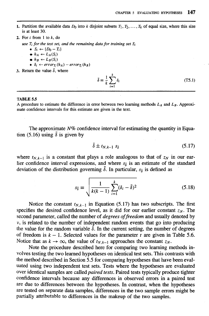
1.
Partition the available data
Do
into
k
disjoint subsets
TI,
T2,
. . .
,
Tk
of equal size, where this size
is at least
30.
2.
For
i
from
1
to
k,
do
use
Ti
for the test set, and the remaining data for training set
Si
0
Si
c
{Do
-
Ti}
hA
C
LA(Si)
h~
+
L~(si)
0
Si
t
errorq
(hA)
-
errorz
(hB)
3.
Return the value
6,
where
TABLE
5.5
A
procedure to estimate the difference in error between two learning methods
LA
and
LB.
Approxi-
mate confidence intervals for this estimate are given in the text.
The approximate
N%
confidence interval for estimating the quantity in Equa-
tion (5.16) using
8
is given by
where
tN,k-l
is a constant that plays a role analogous to that of
ZN
in our ear-
lier confidence interval expressions, and where
s,-
is an estimate of the standard
deviation of the distribution governing
8.
In particular,
sg
is defined as
Notice the constant
t~,k-l
in Equation (5.17) has two subscripts. The first
specifies the desired confidence level, as it did for our earlier constant
ZN.
The
second parameter, called the number of
degrees
of
freedom
and usually denoted by
v,
is related to the number of independent random events that go into producing
the value for the random variable
8.
In the current setting, the number of degrees
of freedom is
k
-
1. Selected values for the parameter
t
are given in Table 5.6.
Notice that as
k
+
oo,
the value of
t~,k-l
approaches the constant
ZN.
Note the procedure described here for comparing two learning methods in-
volves testing the two learned hypotheses on identical test sets. This contrasts with
the method described in Section 5.5 for comparing hypotheses that have been eval-
uated using two independent test sets. Tests where the hypotheses are evaluated
over identical samples are called
paired tests.
Paired tests typically produce tighter
confidence intervals because any differences in observed errors in a paired test
are due to differences between the hypotheses. In contrast, when the hypotheses
are tested on separate data samples, differences in the two sample errors might be
partially attributable to differences in the makeup of the two samples.
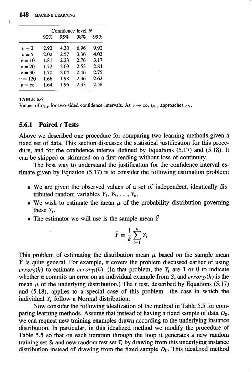
Confidence level
N
90% 95% 98% 99%
TABLE
5.6
Values
oft^,"
for two-sided confidence intervals. As
v
+
w,
t~,"
approaches
ZN.
5.6.1
Paired
t
Tests
Above we described one procedure for comparing two learning methods given a
fixed set of data. This section discusses the statistical justification for this proce-
dure, and for the confidence interval defined by Equations (5.17) and (5.18). It
can be skipped or skimmed on a first reading without loss of continuity.
The best way to understand the justification for the confidence interval es-
timate given by Equation (5.17) is to consider the following estimation problem:
0
0
a
This
We are given the observed values of a set of independent, identically dis-
tributed random variables YI, Y2,
.
.
.
,
Yk.
We wish to estimate the mean
p
of the probability distribution governing
these
Yi.
The estimator we will use is the sample mean
Y
problem of estimating the distribution mean
p
based on the sample mean
Y
is quite general. For example, it covers the problem discussed earlier of using
errors(h) to estimate errorv(h). (In that problem, the
Yi
are 1 or
0
to indicate
whether h commits an error on an individual example from
S,
and errorv(h) is the
mean
p
of the underlying distribution.) The
t
test, described by Equations (5.17)
and (5.18), applies to a special case of this problem-the case in which the
individual
Yi
follow a Normal distribution.
Now consider the following idealization of the method in Table
5.5
for com-
paring learning methods. Assume that instead of having a fixed sample of data Do,
we can request new training examples drawn according to the underlying instance
distribution. In particular, in this idealized method we modify the procedure of
Table
5.5
so that on each iteration through the loop it generates a new random
training set
Si
and new random test set
Ti
by drawing from this underlying instance
distribution instead of drawing from the fixed sample
Do.
This idealized method