Mitchell Т. Machine learning

Подождите немного. Документ загружается.

CHAPTER

ARTIFICIAL

NEURAL

NETWORKS

index (e.g., an integer) is assigned to each node in the network,where

a "node" is either an input to the network or the output of some unit in the

network.

xji

denotes the input from node

to unit

and

wji

denotes the corresponding

weight.

denotes the error term associated with unit

It plays a role analogous

to the quantity

in our earlier discussion of the delta training rule. As

we shall see later,

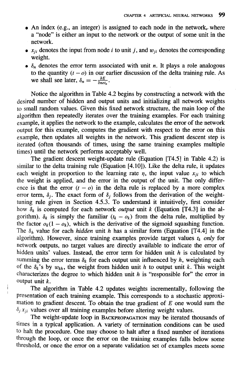
Notice the algorithm in Table 4.2 begins by constructing a network with the

desired number of hidden and output units and initializing all network weights

to small random values. Given this fixed network structure, the main loop of the

algorithm then repeatedly iterates over the training examples. For each training

example, it applies the network to the example, calculates the error of the network

output for this example, computes the gradient with respect to the error on this

example, then updates all weights in the network. This gradient descent step is

iterated (often thousands of times, using the same training examples multiple

times) until the network performs acceptably well.

The gradient descent weight-update rule (Equation

[T4.5] in Table 4.2) is

similar to the delta training rule (Equation [4.10]). Like the delta rule, it updates

each weight in proportion to the learning rate

r],

the input value

xji

to which

the weight is applied, and the error in the output of the unit. The only differ-

ence is that the error

in the delta rule is replaced by a more complex

error term,

aj.

The exact form of

follows from the derivation of the weight-

tuning rule given in Section 4.5.3. To understand it intuitively, first consider

how

is computed for each network

output

unit

(Equation [T4.3] in the al-

gorithm).

is simply the familiar

(tk

ok)

from the delta rule, multiplied by

the factor

ok(l

ok),

which is the derivative of the sigmoid squashing function.

The

value for each

hidden

unit

has a similar form (Equation [T4.4] in the

algorithm). However, since training examples provide target values

only

for

network outputs, no target values are directly available to indicate the error of

hidden units' values. Instead, the error term for hidden unit

is calculated by

summing the error terms

for each output unit influenced by

weighting each

the

ak's

wkh,

the weight from hidden unit

to output unit

This weight

characterizes the degree to which hidden unit

is "responsible for" the error in

output unit

The algorithm in Table 4.2 updates weights incrementally, following the

Presentation of each training example. This corresponds to a stochastic approxi-

mation to gradient descent. To obtain the true gradient of

one would sum the

x,,

values over all training examples before altering weight values.

The weight-update loop in BACKPROPAGATION may be iterated thousands of

times in a typical application. A variety of termination conditions can

used

to halt the procedure. One may choose to halt after a fixed number of iterations

through the loop, or once the error on the training examples falls below some

threshold, or once the error on a separate validation set of examples meets some

100

MACHINE

LEARNING

criterion. The choice of termination criterion is an important one, because too few

iterations can fail to reduce error sufficiently, and too many can lead to overfitting

the training data. This issue is discussed in greater detail in Section 4.6.5.

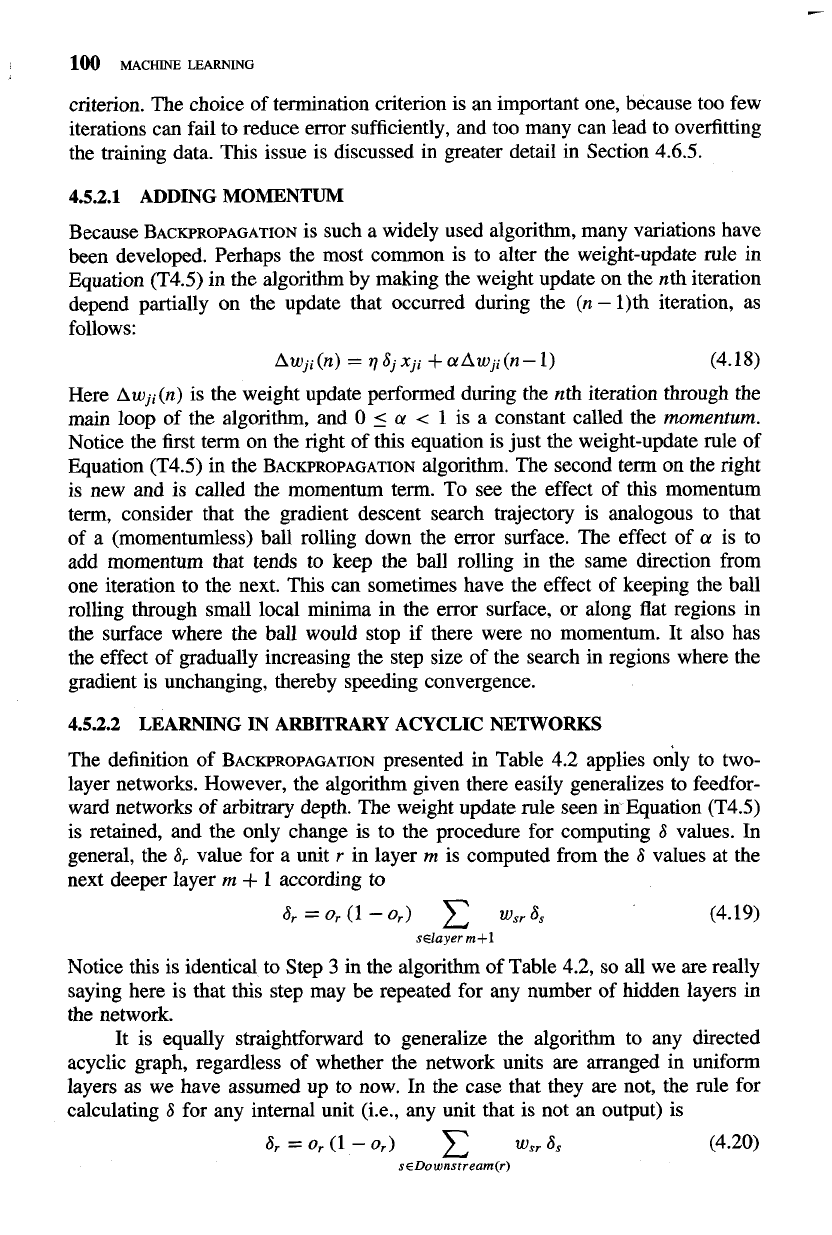
4.5.2.1 ADDING MOMENTUM

Because

BACKPROPAGATION

is such a widely used algorithm, many variations have

been developed. Perhaps the most common is to alter the weight-update rule in

Equation (T4.5) in the algorithm by making the weight update on the nth iteration

depend partially on the update that occurred during the (n

1)th iteration, as

follows:

Here

Awji(n) is the weight update performed during the nth iteration through the

main loop of the algorithm, and

is a constant called the momentum.

Notice the first term on the right of this equation is just the weight-update rule of

Equation (T4.5) in the

BACKPROPAGATION

algorithm. The second term on the right

is new and is called the momentum term. To see the effect of this momentum

term, consider that the gradient descent search trajectory is analogous to that

of a (momentumless) ball rolling down the error surface. The effect of

is to

add momentum that tends to keep the ball rolling in the same direction from

one iteration to the next. This can sometimes have the effect of keeping the ball

rolling through small local minima in the error surface, or along flat regions in

the surface where the ball would stop if there were no momentum. It also has

the effect of gradually increasing the step size of the search in regions where the

gradient is unchanging, thereby speeding convergence.

4.5.2.2 LEARNING

ARBITRARY ACYCLIC NETWORKS

The definition of

BACKPROPAGATION

presented in Table 4.2 applies ohy to two-

layer networks. However, the algorithm given there easily generalizes to feedfor-

ward networks of arbitrary depth. The weight update rule seen in Equation (T4.5)

is retained, and the only change is to the procedure for computing

values. In

general, the

value for a unit

in layer

is computed from the

values at the

next deeper layer

according to

Notice this is identical to Step

in the algorithm of Table 4.2, so all we are really

saying here is that this step may be repeated for any number of hidden layers in

the network.

It is equally straightforward to generalize the algorithm to any directed

acyclic graph, regardless of whether the network units are arranged in uniform

layers as we have assumed up to now.

the case that they are not, the rule for

calculating

for any internal unit (i.e., any unit that is not an output) is

CHAPTER

ARTIFICIAL

NEURAL

NETWORKS

101

where

Downstream(r)

is the set of units immediately downstream from unit

the network: that is, all units whose inputs include the output of unit

It is this

gneral form of the weight-update rule that we derive in Section

4.5.3.

4.5.3

Derivation of the

BACKPROPAGATION

Rule

This section presents the derivation of the

BACKPROPAGATION

weight-tuning rule.

It may be skipped on a first reading, without loss of continuity.

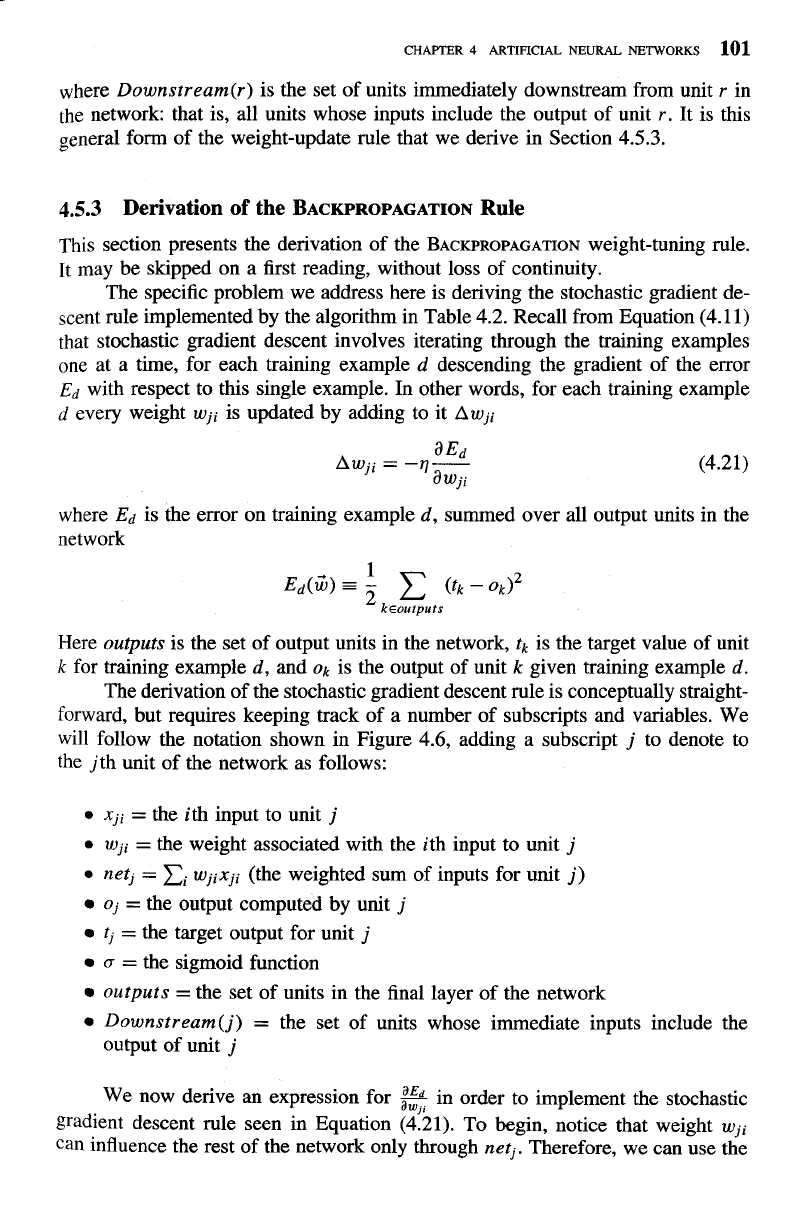
The specific problem we address here is deriving the stochastic gradient de-

scent rule implemented by the algorithm in Table

4.2.

Recall from Equation

(4. ll)

that stochastic gradient descent involves iterating through the training examples

one at a time, for each training example d descending the gradient of the error

with respect to this single example. In other words, for each training example

every weight

wji

is updated by adding to it

Awji

where

is the error on training example d, summed over all output units in the

network

Here

outputs

is the set of output units in the network,

is the target value of unit

for training example d, and

is the output of unit

given training example d.

The derivation of the stochastic gradient descent rule is conceptually straight-

forward, but requires keeping track of a number of subscripts and variables. We

will follow the notation shown in Figure

4.6,

adding a subscript

to denote to

the jth unit of the network as follows:

xji

the ith input to unit

wji

the weight associated with the ith input to unit

netj

wjixji

(the weighted sum of inputs for unit

the output computed by unit

the target output for unit

the sigmoid function

outputs

the set of units in the final layer of the network

Downstream(j)

the set of units whose immediate inputs include the

output of unit

We now derive an expression for

in order to implement the stochastic

gradient descent rule seen in Equation

(4:2l).

To begin, notice that weight

wji

can

influence the rest of the network only through

netj.

Therefore, we can use the

102

MACHINE

LEARNING

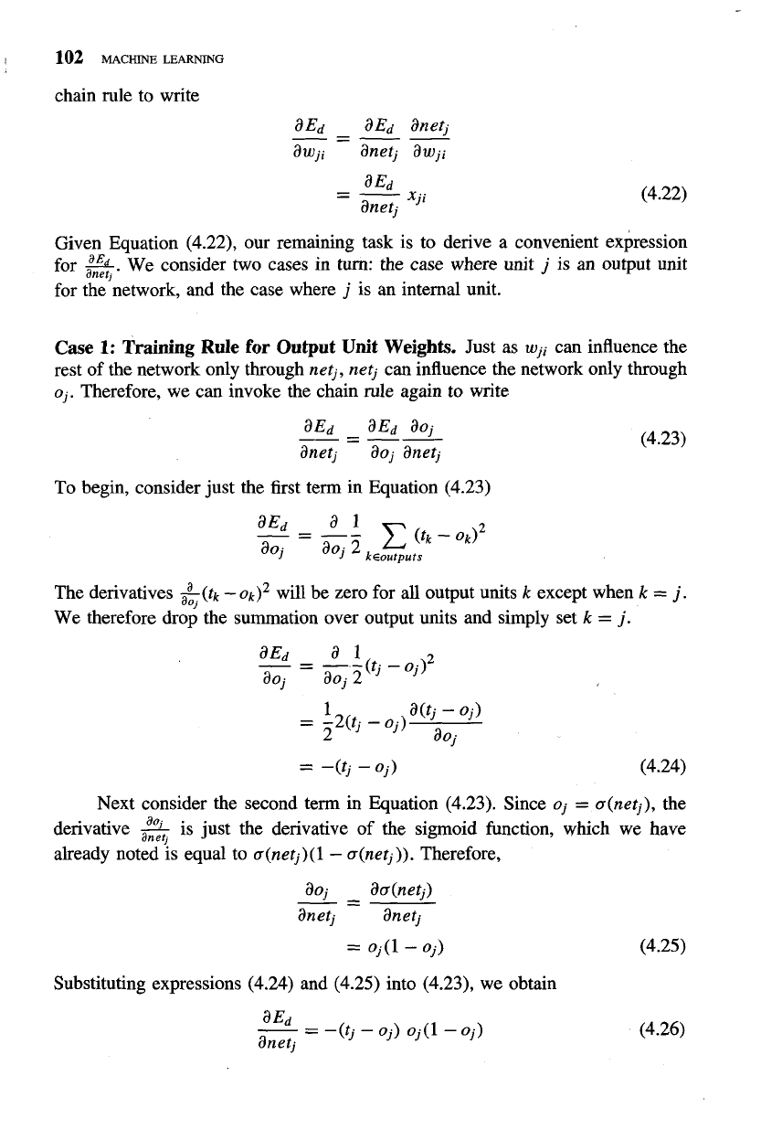
chain rule to write

Given Equation

(4.22),

our remaining task is to derive a convenient expression

for

We consider two cases in turn: the case where unit

is an output unit

for the network, and the case where

is an internal unit.

Case

raini in^

Rule

for

Output Unit

Weights.

Just

wji

can influence the

rest of the network only through

net,, net,

can influence the network only through

oj.

Therefore, we can invoke the chain rule again to write

To begin, consider just the first term in Equation

(4.23)

The derivatives

&(tk

ok12

will be zero for all output units

except when

We therefore drop the summation over output units and simply set

Next consider the second term in Equation

(4.23).

Since

a(netj),

the

derivative

is just the derivative of the sigmoid function, which we have

already noted is equal to

a(netj)(l

a(netj)).

Therefore,

Substituting expressions

(4.24)

and

(4.25)

into

(4.23),

we obtain

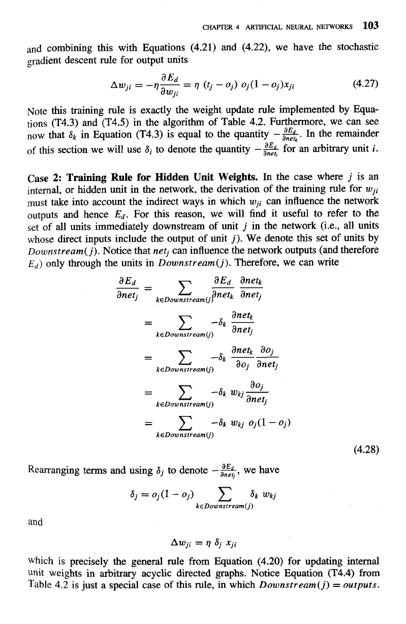
and combining this with Equations (4.21) and (4.22), we have the stochastic

gradient descent rule for output units

Note this training rule is exactly the weight update rule implemented by Equa-

tions (T4.3) and (T4.5) in the algorithm of Table 4.2. Furthermore, we can see

now that

in Equation (T4.3) is equal to the quantity

-$.

the remainder

of this section we will use

to denote the quantity

for an arbitrary unit

Case

Training Rule for Hidden Unit Weights.

In the case where

is an

internal, or hidden unit in the network, the derivation of the training rule for

wji

must take into account the indirect ways in which

wji

can influence the network

outputs and hence

Ed.

For this reason, we will find it useful to refer to the

set of all units immediately downstream of unit

in the network (i.e., all units

whose direct inputs include the output of unit j). We denote this set of units by

Downstream(

j). Notice that

netj

can influence the network outputs (and therefore

Ed)

only through the units in

Downstream(j).

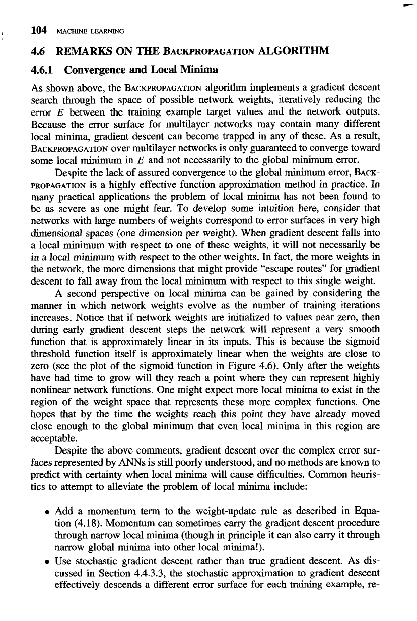
Therefore, we can write

Rearranging terms and using

to denote

-$,

we have

and

which is precisely the general rule from Equation (4.20) for updating internal

unit weights in arbitrary acyclic directed graphs. Notice Equation (T4.4) from

Table

4.2 is just a special case of this rule, in which

Downstream(j)

outputs.

4.6 REMARKS ON THE BACKPROPAGATION ALGORITHM

4.6.1 Convergence

and

Local Minima

As shown above, the BACKPROPAGATION algorithm implements a gradient descent

search through the space of possible network weights, iteratively reducing the

error

between the training example target values and the network outputs.

Because the error surface for multilayer networks may contain many different

local minima, gradient descent can become trapped in any of these. As a result,

BACKPROPAGATION over multilayer networks is only guaranteed to converge toward

some local minimum in

and not necessarily to the global minimum error.

Despite the lack of assured convergence to the global minimum error, BACK-

PROPAGATION

is a highly effective function approximation method in practice. In

many practical applications the problem of local minima has not been found to

be as severe as one might fear. To develop some intuition here, consider that

networks with large numbers of weights correspond to error surfaces in very high

dimensional spaces (one dimension per weight). When gradient descent falls into

a local minimum with respect to one of these weights, it will not necessarily be

in a local minimum with respect to the other weights. In fact, the more weights in

the network, the more dimensions that might provide "escape routes" for gradient

descent to fall away from the local minimum with respect to this single weight.

second perspective on local minima can be gained by considering the

manner in which network weights evolve as the number of training iterations

increases. Notice that if network weights are initialized to values near zero, then

during early gradient descent steps the network will represent a very smooth

function that is approximately linear in its inputs. This is because the sigmoid

threshold function itself is approximately linear when the weights are close to

zero (see the plot of the sigmoid function in Figure

4.6).

Only after the weights

have had time to grow will they reach a point where they can represent highly

nonlinear network functions. One might expect more local minima to exist in the

region of the weight space that represents these more complex functions. One

hopes that by the time the weights reach this point they have already moved

close enough to the global minimum that even local minima in this region are

acceptable.

Despite the above comments, gradient descent over the complex error sur-

faces represented by ANNs is still poorly understood, and no methods are known to

predict with certainty when local minima will cause difficulties. Common heuris-

tics to attempt to alleviate the problem of local minima include:

Add a momentum term to the weight-update rule as described in Equa-

tion (4.18). Momentum can sometimes carry the gradient descent procedure

through narrow local minima (though in principle it can also carry it through

narrow global minima into other local minima!).

Use stochastic gradient descent rather than true gradient descent. As dis-

cussed in Section 4.4.3.3, the stochastic approximation to gradient descent

effectively descends a different error surface for each training example,

re-

CHAPTER

ARTIFICIAL

NEURAL

NETWORKS

105

lying on the average of these to approximate the gradient with respect to the

full training set. These different error surfaces typically will have different

local minima, making it less likely that the process will get stuck in any one

of them.

Train multiple networks using the same data, but initializing each network

with different random weights.

the different training efforts lead to dif-

ferent local minima, then the network with the best performance over a

separate validation data set can be selected. Alternatively, all networks can

be retained and treated as a "committee" of networks whose output is the

(possibly weighted) average of the individual network outputs.

4.6.2

Representational Power of Feedforward Networks

What set of functions can be represented by feedfonvard networks? Of course

the answer depends on the width and depth of the networks. Although much is

still unknown about which function classes can be described by which types of

networks, three quite general results are known:

Boolean functions.

Every boolean function can be represented exactly by

some network with two layers of units, although the number of hidden units

required grows exponentially in the worst case with the number of network

inputs. To see how this can be done, consider the following general scheme

for representing an arbitrary boolean function: For each possible input vector,

create a distinct hidden unit and set its weights so that it activates if and only

if this specific vector is input to the network. This produces a hidden layer

that will always have exactly one unit active. Now implement the output

unit as an OR gate that activates just for the desired input patterns.

Continuous functions.

Every bounded continuous function can be approxi-

mated with arbitrarily small error (under a finite norm) by a network with

two layers of units (Cybenko 1989; Hornik et al. 1989). The theorem in

this case applies to networks that use sigmoid units at the hidden layer and

(unthresholded) linear units at the output layer. The number of hidden units

required depends on the function to be approximated.

Arbitraryfunctions.

Any function can be approximated to arbitrary accuracy

by a network with three layers of units (Cybenko 1988). Again, the output

layer uses linear units, the two hidden layers use sigmoid units, and the

number of units required at each layer is not known in general. The proof

of this involves showing that any function can be approximated by a lin-

ear combination of many localized functions that have value

everywhere

except for some small region, and then showing that two layers of sigmoid

units are sufficient to produce good local approximations.

These results show that limited depth feedfonvard networks provide a very

expressive hypothesis space for BACKPROPAGATION. However, it is important to

keep in mind that the network weight vectors reachable by gradient descent from

the initial weight values may not include all possible weight vectors. Hertz et al.

(1991) provide a more detailed discussion of the above results.

4.6.3 Hypothesis Space Search and Inductive Bias

It is interesting to compare the hypothesis space search of BACKPROPAGATION to

the search performed by other learning algorithms. For BACKPROPAGATION, every

possible assignment of network weights represents a syntactically distinct hy-

pothesis that in principle can be considered by the learner. In other words, the

hypothesis space is the n-dimensional Euclidean space of the n network weights.

Notice this hypothesis space is continuous, in contrast to the hypothesis spaces

of decision tree learning and other methods based on discrete representations.

The fact that it is continuous, together with the fact that

is differentiable with

respect to the continuous parameters of the hypothesis, results in a well-defined

error gradient that provides a very useful structure for organizing the search for

the best hypothesis. This structure is quite different from the general-to-specific

ordering used to organize the search for symbolic concept learning algorithms,

or the simple-to-complex ordering over decision trees used by the ID3 and

C4.5

algorithms.

What is the inductive bias by which BACKPROPAGATION generalizes beyond

the observed data? It is difficult to characterize precisely the inductive bias of

BACKPROPAGATION learning, because it depends on the interplay between the gra-

dient descent search and the way in which the weight space spans the space of

representable functions. However, one can roughly characterize it as smooth in-

terpolation between data points. Given two positive training examples with no

negative examples between them,

BACKPROPAGATION will tend to label points in

between as positive examples as well. This can be seen, for example, in the de-

cision surface illustrated in Figure

4.5,

in which the specific sample of training

examples gives rise to smoothly varying decision regions.

4.6.4 Hidden Layer Representations

One intriguing property of BACKPROPAGATION is its ability to discover useful in-

termediate representations at the hidden unit layers inside the network. Because

training examples constrain only the network inputs and outputs, the weight-tuning

procedure is free to set weights that define whatever hidden unit representation is

most effective at minimizing the squared error

This can lead BACKPROPAGATION

to define new hidden layer features that are not explicit in the input representa-

tion, but which capture properties of the input instances that are most relevant to

learning the target function.

Consider, for example, the network shown in Figure

4.7.

Here, the eight

network inputs are connected to three hidden units, which are in turn connected

to the eight output units. Because of this structure, the three hidden units will

be forced to re-represent

the

eight input values in some way that captures their

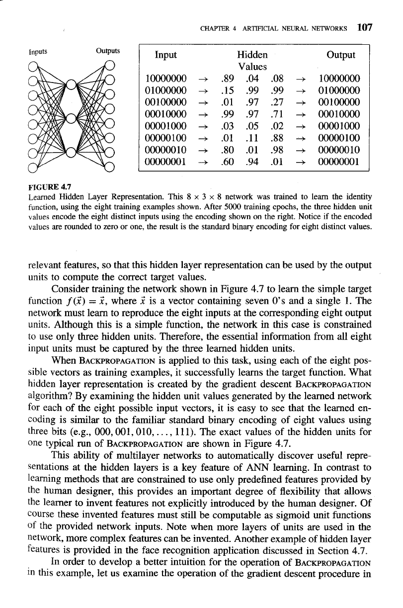
Inputs

Outputs

Input

10000000

0 1000000

00 100000

00010000

00001000

00000 100

ooOOOo

0000000 1

Hidden

Values

.89

.04

.08

.15

.99

.01

.97

.27

.99

.97

.71

.03

.05

.02

.01

.ll

.88

.80

.01

.98

.60

.94

.01

output

10000000

0 1000000

00 100000

000 10000

0000 1000

00000 100

000000 10

0000000 1

FIGURE

4.7

Learned Hidden Layer Representation. This

network was trained to learn the identity

function, using the eight training examples shown. After

5000

training epochs, the three hidden unit

values encode the eight distinct inputs using the encoding shown on the right. Notice if the encoded

values are rounded to zero or one, the result is the standard binary encoding for eight distinct values.

relevant features, so that this hidden layer representation can be used by the output

units to compute the correct target values.

Consider training the network shown in Figure

4.7

to learn the simple target

function

(2)

where

is a vector containing seven

0's

and a single

The

network must learn to reproduce the eight inputs at the corresponding eight output

units. Although this is a simple function, the network in this case is constrained

to use only three hidden units. Therefore, the essential information from all eight

input units must be captured by the three learned hidden units.

When

BACKPROPAGATION is applied to this task, using each of the eight pos-

sible vectors as training examples, it

successfully learns the target function. What

hidden layer representation is created by the gradient descent BACKPROPAGATION

algorithm? By examining the hidden unit values generated by the learned network

for each of the eight possible input vectors, it is easy to see that the learned en-

coding is similar to the familiar standard binary encoding of eight values using

three bits

(e.g.,

000,001,010,.

. .

111).

The exact values of the hidden units for

one typical run of BACKPROPAGATION are shown in Figure

4.7.

This ability of multilayer networks to automatically discover useful repre-

sentations at the hidden layers is a key feature of

ANN

learning. In contrast to

learning methods that are constrained to use only predefined features provided by

the human designer, this provides an important degree of flexibility that allows

the learner to invent features not explicitly introduced by the human designer. Of

course these invented features must still be computable as sigmoid unit functions

of the provided network inputs. Note when more layers of units are used in the

network, more complex features can be invented. Another example of hidden layer

features is provided in the face recognition application discussed in Section

4.7.

order to develop a better intuition for the operation of BACKPROPAGATION

in this example, let us examine the operation of the gradient descent procedure in

greater detailt. The network in Figure

4.7

was trained using the algorithm shown

in Table

4.2,

with initial weights set to random values in the interval (-0.1,0.1),

learning rate

0.3, and no weight momentum (i.e.,

0). Similar results

were obtained by using other learning rates and by including nonzero momentum.

The hidden unit encoding shown in Figure

4.7

was obtained after 5000 training

iterations through the outer loop of the algorithm (i.e., 5000 iterations through each

of the eight training examples). Most of the interesting weight changes occurred,

however, during the first 2500 iterations.

We can directly observe the effect of

BACKPROPAGATION'S gradient descent

search by plotting the squared output error as a function of the number of gradient

descent search steps. This is shown in the top plot of Figure

4.8.

Each line in

this plot shows the squared output error summed over all training examples, for

one of the eight network outputs. The horizontal axis indicates the number of

iterations through the outermost loop of the BACKPROPAGATION algorithm. As this

plot indicates, the sum of squared errors for each output decreases as the gradient

descent procedure proceeds, more quickly for some output units and less quickly

for others.

The evolution of the hidden layer representation can be seen in the second

plot of Figure

4.8.

This plot shows the three hidden unit values computed by the

learned network for one of the possible inputs (in particular, 01000000). Again, the

horizontal axis indicates the number of training iterations. As this plot indicates,

the network passes through a number of different encodings before converging to

the final encoding given in Figure

4.7.

Finally, the evolution of individual weights within the network is illustrated

in the third plot of Figure

4.8.

This plot displays the evolution of weights con-

necting the eight input units (and the constant

bias input) to one of the three

hidden units. Notice that significant changes in the weight values for this hidden

unit coincide with significant changes in the hidden layer encoding and output

squared errors. The weight that converges to a value near zero in this case is the

bias weight

wo.

4.6.5

Generalization, Overfitting, and Stopping Criterion

In the description of t'le BACKPROPAGATION algorithm in Table

4.2,

the termination

condition for the algcrithm has been left unspecified. What is an appropriate con-

dition for terrninatinp the weight update loop? One obvious choice is to continue

training until the errcr

on the training examples falls below some predetermined

threshold. In fact, this is a poor strategy because BACKPROPAGATION is suscepti-

ble to overfitting the training examples at the cost of decreasing generalization

accuracy over other unseen examples.

To see the dangers of minimizing the error over the training data, consider

how the error

varies with the number of weight iterations. Figure

4.9

shows

t~he source code to reproduce this example is available at

http://www.cs.cmu.edu/-tom/mlbook.hhnl.