Mellouk A., Chebira A. (eds.) Machine Learning
Подождите немного. Документ загружается.

Similarity Discriminant Analysis
103
are formally the same for local SDA, except that the mean is computed from the neighbors
of test sample x rather than the whole training set. Thus, the optimized parameters
λ
gh
and
γ
gh
are local. Given the set of local class centroids {µ
h
}, the local class priors
ˆ
P
(Y = g), and
the local class-conditional model parameters γ
gh
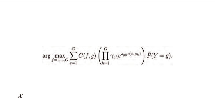
the local SDA classification rule is identical
to the SDA rule (12):
A problem can occur if the hth class has few training samples in the neighborhood of test
sample x. In this case, the local SDA model for class h is difficult to estimate. To avoid this
problem, if the number of local training samples in any of the classes is very small, for
example n
h
< 3, the local SDA classifier reverts to the local nearest centroid classifier. If n
h
= 0
so that
h
is the empty set, then the probability of class h is locally zero, and that class is not
considered in the classification rule (12). This strategy enables local SDA to gracefully
handle small k and very small class priors.
Local classification algorithms have traditionally been weighted voting methods, including
classifying with local linear regression, which can be formulated as a weighted voting
method (Hastie et al., 2001). These methods are by their nature non-parametric and their use
arises in situations when the available training samples are too few to accurately build class
models. On the other hand, it is known that the number of training samples required by
nonparametric classifiers to achieve low error rates grows exponentially with the number of
features (Mitani & Hamamoto, 2006). Thus, when only small training sets are available,
nonparametric classifiers are negatively impacted by outliers. In 2000, Mitani and
Hamamoto (Mitani & Hamamoto, 2000, 2006) were the first ones to propose a classifier that
is both model-based and local. However, they did not develop it as a local generative
method; instead, they proposed the classifier as a local weighted-distance method. Their
nearest-means classifier can be interpreted as a local QDA classifier with identity
covariances. In experiments with simulated and real data sets, the local nearest-means
classifier was competitive with, and often better than, nearest neighbor, the Parzen classifier,
and an artificial neural network, especially for small training sets and for high dimensional
problems.
Local nearest-means differs from local SDA in several aspects. First, the classifier by Mitani
and Hamamoto in (Mitani & Hamamoto, 2006) learns a metric problem, not a similarity
problem: the class prototypes are the local class-conditional means of the features and a
weighted Euclidean distance is used to classify a test sample as the class of its nearest class
mean. Second, the neighborhood definition is different than the usual k nearest neighbors:
they select k nearest neighbors from each class, so that the total neighborhood size is k ×G.
More recently, it was proposed to apply a support vector machine to the k nearest neighbors
of the test sample (Zhang et al., 2006). The SVM-KNN method was developed to address the
robustness and dimensionality concerns that a²ict nearest neighbors and SVMs. Similarly to
the nearest-means classifier, the SVM-KNN is a hybrid local and global classifier developed
to mitigate the high variance typical of nearest neighbor methods and the curse-of-
dimensionality. However, unlike the nearest means classifier of Mitani and Hamamoto,
which is rooted in Euclidean space, the SVM-KNN can be used with any similarity function,
as it assumes that the class information about the samples is captured by their pairwise
Machine Learning
104
similarities without reference to the underlying feature space. Experiments on benchmark
datasets using various similarity functions showed that SVM-KNN outperforms k-NN and
its variants especially for cases with small training sets and large number of classes. SVM-
KNN differs from local SDA because it is not a generative classifier.
Finally, note that different definitions of neighborhood may be used with local SDA. One
could use the Mitani and Hamamoto (Mitani & Hamamoto, 2006) definition described
above, or radius-based definitions. For example, the neighborhood of a test sample x may be
defined as all the samples that fall within a factor of 1+
α
of its similarity to its most similar
neighbor, and
α
is cross-validated. This work employs the traditional definition of
neighborhood, as the k nearest neighbors.
3.1 Consistency of the local SDA classifier
Generative classifiers with a finite number of model parameters, such as QDA or SDA, will
not asymptotically converge to the Bayes classifier due to the model bias. This section shows
that, like k-NN, the local SDA classifier is consistent such that its expected classification
error E[L] converges to the Bayes error rate L* under the usual asymptotic assumptions that
the number of training samples N → ∞, the neighborhood size k → ∞, but that the
neighborhood size grows relatively slowly such that k=N → 0. First a lemma is proven that
will be used in the proof of the local SDA consistency theorem. Also, the known result that
k-NN is a consistent classifier is reviewed in terms of similarity.
Let the similarity function be s :
× → Ω, where Ω ⊂ R is discrete and let the largest
element of -Ω be termed s
max
. Let X be a test sample and let the training samples {X
1
,X
2
, ...
,X
N
} be drawn identically and independently. Re-order the training samples according to
decreasing similarity and label them {Z
1
,Z
2
, ..., Z
N
} such that Z
k
is the kth most similar
neighbor of X.
Lemma 1 Suppose s(x,Z) = s
max
if and only if x = Z and P(s(x,Z) = s
max
) > 0 where Z is a random
training sample. Then P(s(x,Z
k
) = s
max
) → 1 as k, N →∞ and k/N → 0.
Proof: The proof is by contradiction and is similar to the proof of Lemma 5.1 in (Devroye et
al., 1996). Note that s(x,Z
k
) ≠ s
max
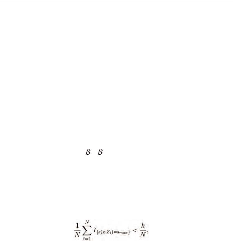
if and only if
(22)
because if there are less than k training samples whose similarity to x is s
max
, the similarity of
the kth training sample to x cannot be s
max
. The left-hand side of (22) converges to P(s(x,Z) =
s
max
) as N→∞ with probability one by the strong law of large numbers, and by assumption
P(s(x,Z) = s
max
) > 0. However, the right-hand side of (22) converges to 0 by assumption.
Thus, assuming s(x,Z
k
) ≠ s
max
leads to a contradiction in the limit. Therefore, it must be that
s(x,Z
k
) = s
max
.
Theorem 1 Assume the conditions of Lemma 1. Define L to be the probability of error for test sample
X given the training sample and label pairs {(Z
1
, Y
1
), (Z
2
, Y
2
), ... , (Z
N
, Y
N
)}, and let L* be the Bayes
error. If k,N → ∞ and k/N → 0, then for the local SDA classifier E[L] → L*.
Proof: By Lemma 1, s(x,Z
i
) = s
max
for i ≤ k in the limit as N → ∞, and thus in the limit the
centroid µ
h
of the subset of the k neighbors that are from class h must satisfy s(x, µ
h
) = s
max
,
for every class h which is represented by at least one sample in the k neighbors. By definition
Similarity Discriminant Analysis
105
of the local SDA algorithm, any class
h that does not have at least one sample in the k
neighbors is assigned the class prior probability P(Y =
h
) = 0, so it is effectively eliminated
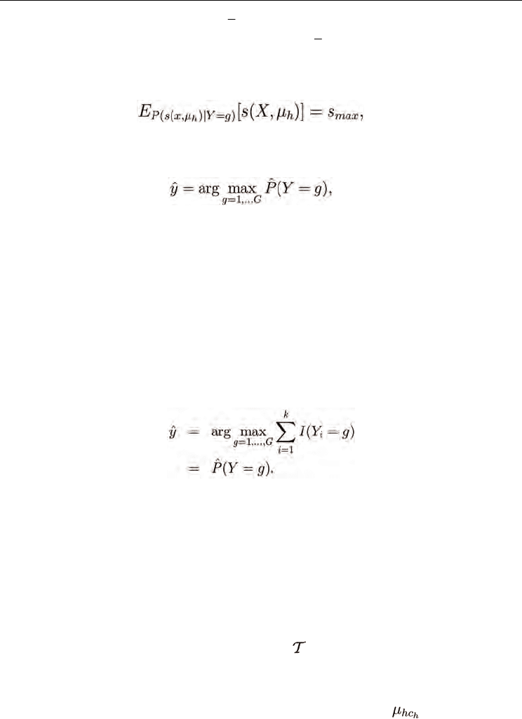
from the possible classification outcomes. Then, the constraint (9) on the expected value of
the class-conditional similarity for every class g that is represented in the k neighbors of x is
(23)
which is solved by the pmf P(s(x, µ
h
)│Y = g) = 1 if s(x, µ
h
) = s
max
, and zero otherwise. Thus
the local SDA classifier (12) becomes
(24)
where the estimated probability of each class
ˆ
P
(Y = g) is calculated using a maximum
likelihood estimate of the class probabilities for the neighborhood. Then,
ˆ
P
(Y = g) →P(Y =
g│x) as k →∞ with probability one by the strong law of large numbers. Thus the local SDA
classifier converges to the Bayes classifier, and the local SDA average error E[L] → L*.
The known result that k-NN is a consistent classifier can be stated in terms of similarity as a
direct consequence of Lemma 1:
Lemma 2 Assume the conditions of Lemma 1 and define L and L* as in Theorem 1. For the
similarity-based k-NN classifier E[L] →L*.
Proof. It follows directly from Lemma 1 that within the size-k neighborhood of x, Z
i
= x for i
≤k. Thus, the k-NN classifier (1) estimates the most frequent class among the k samples
maximally similar to x:
The summation converges to the class prior P(Y = g→x) as k →∞ with probability one by the
strong law of large numbers, and the k-NN classifier becomes that in (24). Thus the
similarity-based k-NN classifier is consistent.
4. Mixture SDA
Like LDA and QDA, basic SDA may be too biased if the similarity space - or more generally
the descriptive statistics space - is multi-modal. In analogy to metric space mixture models,
the bias problem in similarity space may be alleviated by generalizing the SDA formulation
with similarity-based mixture models. In the mixture SDA models, the class-conditional
probability distribution of the descriptive statistics
(x) for a test sample x is modeled as a
weighted sum of exponential components. Generalizing the single centroid-based SDA
classifier and drawing from the metric mixture models (Duda et al., 2001; Hastie et al., 2001),
each class h is characterized by c
h
centroids {µ
hl
}. The descriptive statistics for test sample x
are its similarities to the centroids of class h, {s(x, µ
h1
), s(x, µ
h2
), ... , s(x, )}, for each class h.
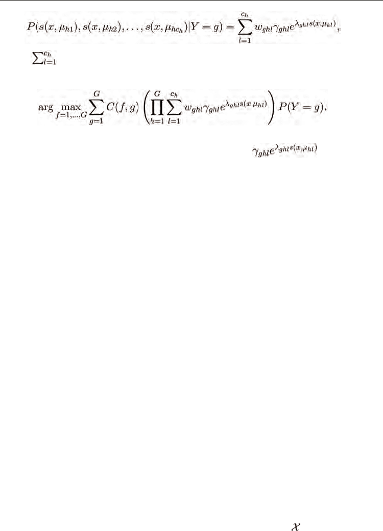
The mixture SDA model for the probability of the similarities, assuming that test sample x is
drawn from class g, is written as
Machine Learning
106
(25)
where
w
ghl
= 1 and w
ghl
> 0. Then, the SDA classification rule (12) for mixture SDA
becomes to classify x as the class
ˆ
y
that solves the maximum a posteriori problem
(26)
Note how the mixture SDA generative model (25) parallels the metric mixture formulation
of Gaussian mixture models (GMMs), with the exponentials
in place of the
Gaussian components. However, there are deep differences between mixture SDA and
metric mixture models. In metric learning, the mixtures model the underlying generative
probability distributions of the features. Due to the curse of dimensionality, high-
dimensional, multi-modal feature spaces require many training samples for robust model
parameter estimation. For example, for d features, GMMs require that a d × 1 mean vector
and a d × d covariance matrix be estimated for each component in each class, for a total of
c
h
×(d
2
+3d)/2 parameters per mixture. Constraining each Gaussian covariance to be diagonal,
at the cost of an increased number of mixture components, alleviates the robust estimation
problem, but does not solve it (Reynolds & Rose, 1995).
When relatively few training samples are available, robust parameter estimation becomes
particularly di±cult. In similarity-based learning the modeled quantity is the similarity of a
sample to a class centroid. The estimation problem is essentially univariate and reduces to
estimating the exponent
λ
ghl
in each component of the mixture, for a total of c
h
× G × 2
parameters per mixture (the scaling parameter γ
ghl
follows trivially). This simpler classifier
architecture allows robust parameter estimation from smaller training set depending on the
number of centroids per class, or, more generally, the number of descriptive statistics.
Another major difference between mixture SDA and metric mixture models is in the number
of class-conditional probability models that must be estimated. In metric learning, G
mixtures are estimated, one for each of the G possible classes from which a sample x may be
drawn. In mixture SDA, G
2
mixture models are estimated. Each sample x is hypothesized
drawn from class g = 1, 2, ...G, and its similarities to each of the G classes are modeled by the
mixture (25), with h = 1, 2. ...G. When the number of classes grows, or when the number of
components in each mixture model grows, the quadratic growth in the number of needed
models presents a challenge in robust parameter estimation, especially when the number of
available training samples is relatively small. However, this problem is mitigated by the fact
that the component SDA parameters may be robustly estimated with smaller training sets
than in metric mixture models due to the simpler, univariate estimation problem at the heart
of SDA classification. The next section discusses the mixture SDA parameter estimation
procedure.
4.1 Estimating the parameters for mixture SDA models
Computing the SDA mixture model for the similarities of samples x ∈
g
to class h requires
estimating the number of components c
h
, the component centroids {µ
hl
}, the component

Similarity Discriminant Analysis
107
weights {w
ghl
} and the component SDA parameters {
λ
ghl
} and {γ
ghl
}. This section describes an
EM algorithm for estimating these mixture parameters. The algorithm parallels the EM
approach for estimating GMM parameters (Duda et al., 2001; Hastie et al., 2001); it is first
summarized below, and then explained in detail in the following sections.
Let
θ
gh
= {{w
ghl
}, {γ
ghl
}, {
λ
ghl
}} for l = 1, 2 ... c
h
be the set of parameters for the class h mixture
model to be estimated under the assumption that the training samples z
i
, for i = 1, 2, ... n
g
are
drawn identically and independently. Denote by C a random component of the mixture and
by P(C = l│s(z
i
, µ
hl
),
θ
gh
) the responsibility (Hastie et al., 2001) of the lth component for the
ith training sample similarity s(z
i
, µ
hl
). Also write P(s(z
i
, µ
hl
)│C = l,
θ
gh
) = .
The proposed EM algorithm for mixture SDA is:
1. Compute the centroids {µ
hl
} with K-medoids algorithm.
2. Initialize the parameters {w
ghl
} and the components P(s(z
i
, µ
hl
)│C = l,
θ
gh
).
3. E step: compute the responsibilities
(27)
4. M step: compute model parameters
(a) Find the
λ
ghl
which solves
(28)
(b) Compute the corresponding scaling factor
(29)
(c) Compute the component weights
(30)
5. Repeat E and M steps until convergence criterion is satisfied.
Note that, just like EM for GMMs, the EM algorithm for mixture SDA involves iterating the
E step, which estimates the responsibilities, and the M step, which estimates the parameters
that maximize the expected log-likelihood of the training data. At each iteration of the M
step, the explicit expression (30) updates the component weights. However, unlike EM for
GMMs, the update expression for the component parameters (28) is implicit and must be
solved numerically. Another difference between the GMM and SDA EM algorithms is in
how the centroids are estimated. For GMMs, the component means {u
hl
}, which are the
metric centroids, are updated at each iteration of the M step. For mixture SDA, the centroids
{µ
hl
} are estimated at the beginning of the algorithm and kept constant throughout the
iterations.
Machine Learning
108
The update expressions for the mixture SDA parameters are derived from the expression of
the expected log-likelihood of the observed similarities. A standard assumption in EM is
that the observed data are independent and identically distributed given the class and
mixture component. For mixture SDA, this assumption means that the training sample
similarities {
g
(z
i
)} = {s(z
i
, µ
hl
)}, z
i
∈
g
to the component centroids are identically
distributed and conditionally independent given the lth class component. Then, the
expected log-likelihood of {
g
(z
i
)} is
(31)
Using the properties of the logarithm and rearranging the terms, L({
g
(z
i
)}│
θ
gh
) splits into
the terms depending on w
ghl
and the terms depending on
λ
ghl
and γ
ghl
:
(32)
The standard EM approach to maximizing (32) is to set its partial derivatives with respect to
the parameters to zero and solve the resulting equations. This is the approach adopted here
for estimating the mixture SDA parameters
θ
gh
for all g, h.
The derivation of the expression for the component weights {w
ghl
} follows directly from (32);
both the derivation of and the final expression for the component weights are identical to
the metric mixtures case. Section 4.1.1 re-derives the well-known expression for w
ghl
.
Applying the EM approach, however, does not lead to explicit expressions for {
λ
ghl
} and
{γ
ghl
}. Instead, it leads to many single-parameter constraint expressions for the mean
similarities of the training data to the mixture component centroids. These expressions are
solved with the same numerical solver used in the single-centroid SDA classifier.
4.1.1 Estimating the component weights
To compute the log-likelihood-maximizing weights w
ghl
, one uses the standard technique of
taking the derivative of the log-likelihood with respect to w
ghl
, setting it to zero, and solving
the resulting expression for w
ghl
. The constraint w
ghl
= 1 is taken into account with the
Lagrange multiplier η:
which gives the well-known expression for the component weights of a mixture model in
terms of the responsibilities:
Similarity Discriminant Analysis
109
(33)
4.1.2 Estimating γ
ghl
and
λ
ghl
The same approach used for estimating the component weights {w
ghl
} is adopted to estimate
the SDA parameters {γ
ghl
} and {
λ
ghl
}: Find the likelihood-maximizing values of the
parameters by setting the corresponding partial derivatives to zero and solving the resulting
equations. First, since each γ
ghl
is simply a scaling factor that ensures that each mixture
component is a probability mass function, one rewrites
(34)
where X ∈
g
is a random sample from class g, s(X, µ
hl
) is its corresponding random
similarity to component centroid µ
hl
, and Ω is the set of all possible similarity values.
Substituting (34) into (32), setting the partial derivative of L({
h
(z
i
)}│
θ
gh
) with respect to
λ
ghl
to zero, and rearranging the terms gives
(35)
The first term on the left side of (35) is simply the definition of the expected value of the
similarity of samples in class g to the lth centroid of class h. Thus, one rewrites (35)
(36)
Expression (36) is an equality constraint on the expected value of the similarity of samples
z
i
∈
g
to the component centroids µ
hl
of class h. This is the same type of constraint that must
be solved in the mean-constrained, maximum entropy formulation of single-centroid SDA
(9). In (9), the mean similarity of samples from class g to the single centroid of class h is
constrained to be equal to the observed average similarity. Analogously, in (36), the mean
similarity of the samples from class g to the lth centroid of class h is constrained to be equal
to the weighted sum of the observed similarities, where each similarity is weighted by its
normalized responsibility. To solve for
λ
ghl
, one uses the same numerical procedure used to
solve (9) and described in Section 2.1. Thus, solving for all the {
λ
ghl
} requires solving the
G ×
c
h
expressions of (36).
It is not surprising that taking the EM approach to estimating
λ
ghl
has lead to the same
expressions for the mean constraints in the maximum entropy approach to density
estimation. It is known that maximum likelihood (ML) - the foundation for EM - and
Machine Learning
110
maximum entropy are dual approaches to estimating distribution parameters which lead to
the same unique solution based on the observed data (Jordan, 20xx). The ML approach
assumes exponential distributions for the similarities, maximizes the likelihood, and arrives
at constraint expressions whose solutions give the desired values for the parameters. The
maximum entropy approach assumes the constraints, maximizes the entropy, and arrives at
exponential distributions whose parameters satisfy the given constraints. This powerful
dual relationship between ML and maximum entropy extends from metric problems to
similarity-based problems; for this reason it leads to the the constraint expression (36), from
which
λ
ghl
is numerically computed. The corresponding γ
ghl
is found by applying (34).
4.1.3 Estimating the centroids
Estimating the centroids of a mixture model encompasses two problems: estimating the
number of components (i.e. centroids) {c
h
}, and estimating the centroids {µ
hl
}. This work
adopts the common metric learning practice of cross-validating the number of mixture
components {c
h
}. The centroids {µ
hl
} are estimated with the K-medoids algorithm (Hastie et
al., 2001), using the maximum-sum-similarity criterion (3). The initial centroids are selected
randomly from the training set samples z
i
∈
h
.
4.1.4 Initializing EM for SDA
In this work, the component weights {w
ghl
} are uniformly initialized to w
ghl
= 1=c
h
and the
components are assigned uniform initial probability P(s(z
i
, µ
hl
)│C = l,
θ
gh
) =
1/c
h
. This
initialization reflects the assumption that initially the mixture components equally
contribute to a sample's class-conditional probability: it is the least-assumptive initialization.
Another strategy would be to initialize the weights by the
fraction of training samples
assigned to the clusters which result from estimating the
centroids with K-medoids. The
component probabilities may also be initialized by
estimating the SDA parameters {
λ
ghl
} and
{γ
ghl
} from the K-medoids clusters. This
is analogous to the GMM initialization strategy
based on the results of the K-means algorithm. In practice, the simple uniform initialization
works well.
5. Experimental results
SDA, local SDA, mixture SDA, and nnSDA are compared to other similarity-based
classifiers in a series of experiments: the tested classifiers are the nearest centroid (NC), local
nearest centroid (local NC), k-nearest neighbors (k-NN) in similarity space, condensed
nearest neighbor (CNN) (Hastie et al., 2001) in similarity space, and the potential support
vector machine (PSVM) (Hochreiter & Obermayer, 2006). When the features underlying the
similarity are available, the classifiers are also compared to the naive Bayes classifier (Hastie
et al., 2001). The counting similarity (the number of features identically shared by two
binary vectors) and the VDM (Stanfill & Waltz, 1986; Cost & Salzberg, 1993; Wilson &
Martinez, 1997) similarities are used to compute the similarities on which the classifiers
operate, except for cases in which similarity is provided as part of benchmark datasets.
The first set of comparisons involves simulated binary data, where each class is generated
by random perturbations of one or two centroids. The perturbed centroids simulation is a
scenario where each class is characterized by one or two prototypical samples (centroids),
but samples have random perturbations that make them different from their class centroid

Similarity Discriminant Analysis
111
in some features. Thus, this simulation fits the centroid- based SDA models, in that each
class is defined by perturbations around one or two prototypical centroids.
Then, three benchmark datasets are investigated: the protein dataset, the voting dataset, and
the sonar dataset. The results on the simulated and benchmark datasets show that the
proposed similarity-based classifiers are effective in classification problems spanning
several application domains, including cases when the similarity measures do not possess
the metric properties usually assumed for metric classifiers and when the underlying
features are unavailable.
For local SDA and local NC, the class prior probabilities are estimated as the empirical
frequency of each class in the neighborhood; for SDA, mixture SDA, nnSDA, NC, and CNN
they are estimated as the empirical frequency of each class in the entire training data set. The
k-NN classifier is implemented in the standard way, with the neighborhood defined by the
test sample’s k most similar training samples, irrespective of the training samples class. Ties
are broken by assigning a test sample to class one.
5.1 Perturbed centroids
In this two-class simulation, each sample is described by d binary features such that
B = {0, 1}
d
. Each class is defined by one or two prototypical sets of features (one or two
centroids). Every sample drawn from each class is a class centroid with some features
possibly changed, according to a feature perturbation probability. Several variants of the
simulation are presented, using different combinations of number of class centroids, feature
perturbation probabilities, and similarity measures. Given samples x, z ∈ B, s(x, z) is either
the counting or the VDM similarity. The simulations span several values for the feature
dimensions d and are run several times to better estimate mean error rates. For each run of
the simulation and for each number of features considered, the neighborhood size k for local
SDA, local NC, and k-NN is determined independently for the three classifiers by leave-one-
out cross-validation on the training set of 100 samples; the range of tested values for k is
{1, 2, ... 20, 29, 39, ... , 99}. The optimum k is then used to classify 1000 test samples. Similarly,
the candidate numbers of components for mixture SDA and for CNN are {2, 3, 4, 5, 7, 10}. To
keep the experiment run time within a manageable practical limit, five-fold cross validation
was used to determine the number of components for mixture SDA, and the mixture SDA
EM algorithm was limited to 30 iterations for each cross-validated mixture model. The
parameters for the PSVM classifier are cross-validated over the range of possible values
ε = {0.1, 0.2, ... 1} and C = {1, 51, 101, ... 951}.
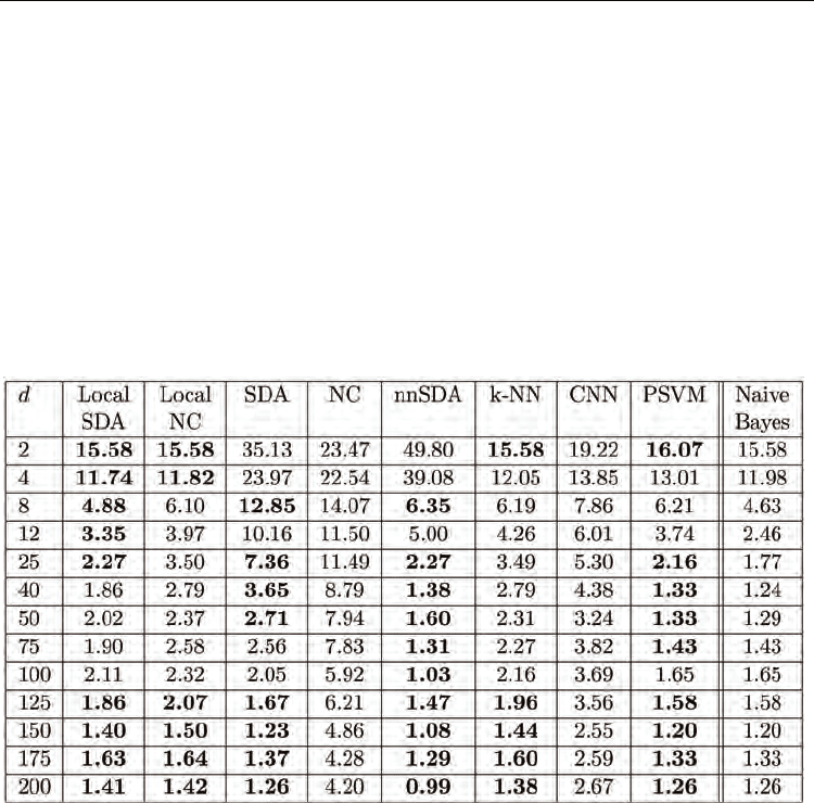
The perturbed centroid simulation results are in Tables 1-8. For each value of d, the lowest
mean cross-validation error rate is in bold. Also in bold for each d are the error rates which
are not statistically significantly different from the lowest mean error rate, as determined by
the Wilcoxon signed rank test for paired differences, with a significance level of 0.05. The
naive Bayes classifier results are also included for reference.
5.1.1 Perturbed centroids – one centroid per class
Each class is generated by perturbing one centroidal sample. There are two, equally likely
classes, and each class is defined by one prototypical set of d binary features, c
1
or c
2
, where
c
1
and c
2
are each drawn uniformly and independently from {0, 1}
d
. A training or test sample
z drawn from class g has the ith feature z[i] = c
g
[i] with probability 1 - p
g
, and z[i] ≠ c
g
[i] with
perturbation probability p
g
. In one set of simulation results p
1
= 1/3 and p
2
= 1/30; thus, class
Machine Learning
112
two is well-clustered around its generating centroid and the two classes are well-separated.
In another set of simulation results, p
1
= 1/3 and p
2
= 1/4 and the two classes are not as well
separated. Classifiers are trained on 100 training samples and tested on 1000 test samples
per run; twenty runs are executed for a total of 20, 000 test samples. The number of features
d ranges from d = 2 to d = 200 in the simulation, but the number of training samples is kept
constant at 100, so that d = 200 is a sparsely populated feature space. This procedure was
repeated for the counting and for the VDM similarities, so there are four sets of results for
the one centroid simulation, depending on the perturbation probabilities and the similarity
measure used. The results are in Tables 1-4.
The performance of all classifiers increases as d increases. For large d, the feature space is
sparsely populated by the training and test samples, which are segregated around their
corresponding generating centroids. This leads to good classification performance for all
classifiers. For small d, the feature space is densely populated by the samples, and the two
classes considerably overlap, negatively affecting the classification performance.
Table 1. Perturbed centroids experiment - One centroid per class. Misclasssification
percentage for counting similarity, perturbation probabilities p
1
= 1/3 and p
2
= 1/30.
Across all four sets of results, the naive Bayes classifier almost always gives the best
performance. Its assumption that the features are independent captures the true underlying
relationship of the sample features makes the naive Bayes classifier well suited for these
particular data sets: indeed the samples are generated as random vectors of independent
binary features. The consequent excellent performance of the naive Bayes classifier provides
a reference point for the other classifiers. More generally, when a classification problem
involves samples natively embedded in an Euclidean space, as in these perturbed centroids
experiments, metric-space classifiers like naive Bayes can perform well. In these cases, the
similarity-based classification framework provides no clear advantage.
On the other hand, naive Bayes cannot be used when the samples are not described by vectors
of independent features, either because the features are not known, the independence
assumption is too restrictive for effective performance, or because the Euclidean