Mei C., Zhou J., Peng X. Simulation and Optimization of Furnaces and Kilns for Nonferrous Metallurgical Engineering

Подождите немного. Документ загружается.

6 Simulation and Optimization of Electric Smelting Furnace 

Table 6.6 Some properties of slag and nickel matte (1250ć)˄Kaiser and Downing 1978˅

Physical

properties

Density

/kg噝

−3

Specific

heat c/J

噝

−1

噝K

−1

Viscosity

/Pa噝s

Kinematic

viscosity

v/m

噝s



Thermal

conductivity

/W噝 m



噝



Thermal

diffusivity

a/m

噝s

−1

Electric

conductivit

/S噝m

−1

Slag 3200 1250 0.3

9.38

h

−5

8.0

2.0

h10

−6

30.0

Nickel

matte

4500 720 0.05

1.11

h

−5

17.0

5.25

h

−6

93.0

Some simplifications are made in order to construct a physical model that

can be manipulated by mathematical method. These include: the electric and

thermal fields of the furnace do not change with time; slag surface and matte

surface stay steadily; and all the electrodes inset to the same depth into the slag.

As the rectangular coordinates are used, the circular electrode can be simplified

to be square electrode with the same conductive area (this will not result in a

big calculation error). The influence of alternating magnetic field on electric

field is neglected (Bochmann et al.,1968)

With the consideration of the

symmetry of the electricity and thermal distributions as well as their influence

on the smelting process, the analytical zone is selected to be either side of the

lateral cross sections of the furnace (Fig. 6.14), and the upper boundary is the

slag surface.

Under the rectangular coordinates, the differential equation of the heat transfer

in the furnace is:

TTT

λλλP

xxyy zz

⎛⎞

∂∂ ∂∂ ∂∂

⎛⎞ ⎛⎞

+++=

⎜⎟

⎜⎟ ⎜⎟

∂∂ ∂∂ ∂∂

⎝⎠ ⎝⎠

⎝⎠

(6.17)

where T is temperature;

λ is thermal conductivity; P is Joule heat, and P=0 in the

lining.

ϕϕϕ

⎡⎤

⎛⎞

∂∂∂

⎛⎞ ⎛⎞

⎢⎥

=++

⎜⎟

⎜⎟ ⎜⎟

⎢⎥

∂∂ ∂

⎝⎠ ⎝⎠

⎝⎠

⎣⎦

P σ

xy z

(6.18)

where

σ is electric conductivity;

is electric potential.

The boundary conditions are as follows. On the central cross section which

divides the furnace symmetrically along its width (

y direction), there is no

normal heat flow. The heat convection and radiation exist between the furnace

lateral wall, as well as the exterior bottom surface, and the environment.

Temperatures of the electrode, furnace chamber, cooling water and furnace raw

charge are known. Other boundary surfaces of the computational domain are

adiabatic.

  Jiemin Zhou and Ping Zhou

For the moving molten slag, its thermal conductivity can be expressed as:

λλ λ=+

where

λ is the thermal conductivity when the slag is immobile, which

represents the heat transfer originated from diffusion and collision of molecules.

λ is the turbulent thermal conductivity when the slag is moving, which

represents the heat transfer originated from micelle mixing and spiral vortex.

According to the similarity between heat transfer and momentum transfer when

the fluid is flowing (Mei, 1987; Zhou, 1991), it can be assumed that Prandtl

number is approximately a constant and irrelevant to the flow pattern of the

continuous medium, that is:

PrĬPr

≈

lpt

μμ

λλ

≈

Therefore,

≈

where

Pr is Prandtl number;

r is turbulent Prandtl number; v

are molecular

and turbulent kinematic viscosity respectively;

a ,

a are molecular and turbulent

thermal diffusivity respectively;

are molecular and turbulent dynamic

viscosity respectively;

is specific heat.

In the research of turbulent flow, there are many ways to evaluate

μ , with

which an approximate value of

can then be obtained.

The electric conduction equation is:

ϕϕϕ

⎛⎞

∂∂ ∂∂ ∂∂

⎛⎞ ⎛⎞

++=

⎜⎟

⎜⎟ ⎜⎟

∂∂∂∂∂∂

⎝⎠ ⎝⎠

⎝⎠

σσσ

xxyyzz

(6.19)

Boundary conditions are as follows. The electric potential of electrode is known.

The normal components of current at the central vertical surface, at the interface

of slag and furnace wall, and at the interfaces of slag and charge as well as furnace

gas are all zero. Other boundaries are zero-potential surfaces.

Because the six electrods are connected to three transformers and the voltages

of the two electrodes in the computational domain are not in the same phase, the

voltage should be decomposed into a horizontal component and a vertical

component firstly, then they will be combined at the end of the calculation in a

geometric way.

Finite difference method is adopted to solve the problem, and the calculation

zone is divided into two parts, using different grids in the analysis of electric and

thermal field respectively.

6 Simulation and Optimization of Electric Smelting Furnace 

6.4.2



Simulation software

The electric and thermal field simulation software of electric smelting furnace

consists of electric field calculation component, temperature field calculation

component and drawing component. The circular iteration method is adopted

to solve such problems as electric conductivity of slag and thermal

conductivity of various refractory and insulation materials varying with

temperature. The unidimensional compression memory technology and

root-squaring method for linear equations are used to solve large scale

differential equation set.

The calculation results can be presented as isopotential lines, isothermal lines,

electric current field, heat flux field on the cross sections and longitudinal section

of the furnace, and can also be plotted as stereo distribution charts of electric

potential, temperature and electric power. The heat balance table, the star current,

delta current and total current of the electrode, the electrode -to-ground resistance,

the electric power, the slag average temperature, the nickel matte average

temperature, the charge consumption per day, and the electricity consumption of

calcine etc. can also be printed out. Sufficient useful information can be obtained

from the simulation.

6.4.3



Calculation results and verification

Simulation is implemented based on the No.2 furnace in Jinchuan Nonferrous

Metal Company, for conditions when the secondary voltage is 400V, electrode

insertion depth is 0.4m, height of nickel matte is 0.75m, slag height is 2.2m, slag

electric conductivity is 30 S/m (Si/Fe ratio in the slag is 1.2, and content of

magnesia is 10.6%), and the distance between the charge and the electrode is 0.4m.

Parts of the calculation results are shown in Fig. 6.15 to Fig. 6.22.

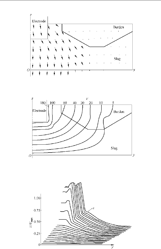
Fig. 6. 15 is the current distribution on the vertical cross section passing the

electrode (sketch of this cross section is shown in Fig. 6.14 (b)), which presents

the relative magnitude and direction of the current. Fig. 6.16 is the isopotential

line on this cross section. It can be seen that the potential gradient is big around

the electrode, but drops smoothly in the region that is far away from the electrode.

Fig. 6.17 is the stereo potential distribution on this cross section, which shows the

variation of electric potential on the whole section more visually. Fig. 6.18 is the

heat flux on the cross section. The heat mainly comes from electricity near the

electrode, and most of the heat flows towards the charge, while some dissipates

through slag surface, cooling water and furnace wall.

  Jiemin Zhou and Ping Zhou

Fig. 6.15 Current distribution on the cross section of furnace

Fig. 6.16 Equipotential lines on the vertical cross section

Fig. 6.17 Electric potential distribution on the cross

section of furnace (

max

=200V)

6 Simulation and Optimization of Electric Smelting Furnace 

Fig. 6.18 Heat flux distribution on the transversal section of furnace

(Vector module of heat flux: 1cm represents 200kW

m

)

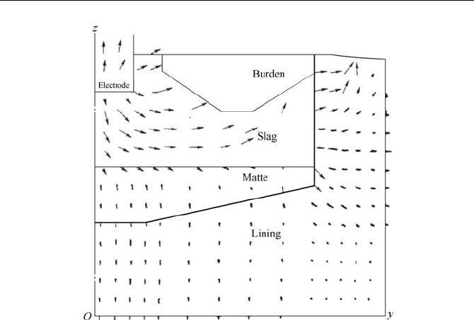
Fig. 6.19 is the isothermal line, which illustrates the variation of temperatures in

the molten pool and lining clearly. By drawing the isothermal lines of the slag and

nickel matte melting points, it can also be examined whether or not the slag is

frozen at furnace wall, or the matte is frozen at the furnace bottom. Fig. 6.20 is the

distribution of the electric power on the cross sections of the furnace. It is obvious

that the power liberated near the electrode is much larger than that in other regions

in the pool, and the power density at the centre of the molten pool is also larger

than that near the lateral wall. Besides, as cross section 1 is a central cross section

between two electrodes which connect to the same transformer, while cross

section 2 is a central section between two electrodes connected to different

transformers, their distributions of power density are different, which is a

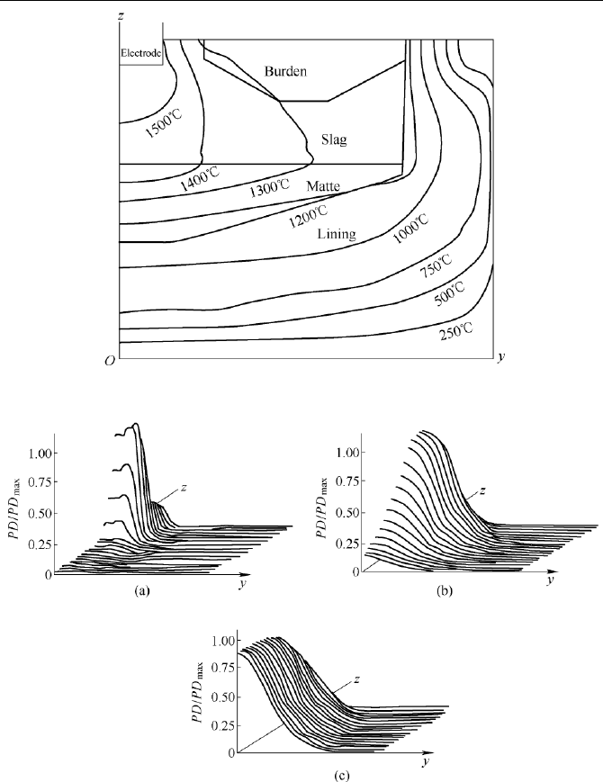
character of six-electrode furnace. Fig. 6.21 is the current distribution on the

longitudinal section near No.2 electrode (between cross section 1 and 2). Because

its voltages and phases to the left and right neighbor electrodes are different, the

current distributions on the two sides are also different. So there are two different

delta currents in the later calculation. This problem has not been mentioned in

previous literatures.

Fig. 6.22 is the distribution of stereo electric potential and power density on

the longitudinal section. It can be seen that the potential distributions are

unsymmetrical on the two sides of the electrode. And it can also be found that

the high power density is located in the region near the bottom of the

electrode.

  Jiemin Zhou and Ping Zhou

Fig. 6.19 Isothermal lines on the cross section of furnace

Fig. 6.20 Power density distribution on the cross section of furnace

(a) Cross section (passing the electrode center), PD

max

=466.4kWm

;

(b) Cross

section 1, PD

max

=46.6kWm

;

max

=21.4kWm

The heat balance of the computational do main that is below the slag surface is

shown in Table 6.7. In this calculation, apparent heat of the calcine, chemical reaction

heat, heat taken away by gas and heat losses through the furnace wall above the slag

are all represented as the heat that is needed to melt calcine and the heat radiated from

the slag surface.

6 Simulation and Optimization of Electric Smelting Furnace 

Fig. 6.21 Current distribution on the longitudinal section of furnace

Fig. 6.22 Electric potential and power density distribution on longitudinal

cross section of furnace

(a) Electric potential distribution, V

max

=200V; (b) Power density distribution, PD

max

=436.8kWgm

-3

Table 6.7 Heat balance of the electric smelting furnace

Item Heat income/kW % Heat expenditure/kW %

Heat supplied by electricity 12369.5 100

Heat used to melt calcine 8851.0 69.1

Heat radiated from slag surface 3309.3 26.80

Heat transferred from electrode 5.9 0.05

Heat taken away by cooling water 229.9 1.9

Heat dissipated from furnace wall 303.2 2.5

(Bottom of furnace) (117.9) (1.0)

(Furnace wall) (185.4) (1.5)

Error

−29.3 −0.2

Total heat 12369.5 100 12369.5 100

Other calculation results are:

  Jiemin Zhou and Ping Zhou

Current in electrode/kA 10.3

Star current/kA 8.7

Delta current (between the two electrodes of the same transformer)/kA 1.3

Delta current (between the two electrodes of different transformers)/kA 0.6

Resistance (electrode to ground) /m

Ω

19.4

Average temperature of slag/

1354

Average temperature of nickel matte/

1169

Charge consumption in every shift/t 171

Electricity consumption per ton calcine/kW

噝h噝t

−1

578.6

To verify the calculation result, a water model test apparatus was made, of

which the size is one fiftieth of the real furnace. KCl solution is used to simulate

the slag, a bottom plane of graphite is used to simulate the nickel matte, and a

wood board is used to simulate the charge. A double-sided compound copper plate

and a bakelite electrode pasted with aluminium foil are used to make an

instrument to measure the current densities in molten pool and electrode. The

influences of pool depth, electrode size, electrode insertion depth and feeding

mode on electric distribution in the liquid pool are measured. In this way, the

electric characteristics of the rectangular six-electrode furnace are revealed

(Zhou,1991). Temperatures from the simulation are verified with the real data

taken from No.2 furnace in Jinchuan Nonferrous Metal Company. Calculation

values of the electric and temperature fields agree well with the measured results.

6.4.4



Evaluation and optimization of the furnace design and

operation

Influences of the secondary voltage of furnace, the insertion depth of electrode, the

way of feeding, the slag thickness, the width of molten pool, the spacing between

electrodes, the electrode diameter, the lining thickness and the electric conductivity

of slag on the furnace production capacity and electricity consumption are examined

by using the electric-thermal analytical model. The quantitative relationship between

the operation condition, design parameters of the nickel electric smelting furnace

and the electricity and heat distributions of the furnace, as well as the main technical

economic indices are established for the first time (Zhou et al., 1991a, b, 1993). It is

then possible to further enhance the furnace productivity and to reduce the energy

consumption by finding the optimum configuration parameters and operation

technical conditions (manual or automatic optimization) according to the simulation

of the software. For No. 2 furnace, there are such optimizations to be made, which

include: improving of feeding way to make the charge cover the high-temperature

slag near the electrode completely so that heat loss can be reduced

ˈmagnifying the

6 Simulation and Optimization of Electric Smelting Furnace 

dimension of furnace body or the depth of charge submerged in the slag to increase

the heat exchange area between the molten slag and charge

ˈ ensuring high

temperature and velocity of the slag to improve the heat transfer intensity on the

interface of molten slag and charge, creating the best temperature field to ensure a

safe production and a long furnace body life while having a high-production and

low-consumption. Referring to the production experience in this factory, some

feasible schemes are also presented for the improvement of production condition of

the furnace. According to the primary optimization that aims for the lowest energy

consumption by using the analytical model, the following schemes can be chosen.

These are, for smelting powder calcine, a uniform and continuous charge

distributing is adopted, so a thin layer charge can cover the exposed slag surface

near the electrode; the length and width of the molten pool is enlarged and then the

area for melting charge can be increased. The specific configuration parameters and

electric regime are as follows :

Width of the molten pool/m 6.20

Spacing between the electrodes/m 3.30

Height of the furnace chamber/m 4.00

Power per square meter /kV

gAgm

−2

113

Secondary voltage/V 360

Insertion depth of electrode/m 0.57

Thickness of slag/m 1.45

Thickness of nickel matte/m 0.75

Thickness of charge/m 0.30

Under the production condition mentioned above, indices as following can be

obtained when the electricity and the charge supply is sufficient:

Electricity consumption per ton calcine/ kWghgt

−1

502

Calcine melted per shift/t 245

Average temperature of slag/

1,334

Average temperature of nickel matte/

1,198

Compared with the production indices of No.2 furnace in 1987, the electricity

consumption is 15% lower, and the charge melted per day increases 19%. The

consumption of such materials as paste and casing are also reduced because the

furnace chamber temperature decreases.

This three-dimensional electric-thermal numerical model and software of the

electric smelting furnace provide a new tool to reasonably choose electric regime

and operation conditions of the smelting process, and to optimize the furnace

configuration design. The model is more practical than that ever reported in

previous research, and to some extends, the information obtained from it covers

  Jiemin Zhou and Ping Zhou

and even surpasses the previous investigations.

This simulation software can be further improved to be a standard program for

testing the design and operation of electric smelting furnace, and provides

systematical data for online optimization control of the furnace (Warczok and

Riverosa, 2007; Guo et al., 2002; Eric, 2004; Pan et al., 2006; Wang et al., 2006).

References

Ambrosio P D et al (1981) Temperature and internal stress distribution of carbon electrodes

used in an electric arc furnace for the production of silicon metal. High

Temperatures-High Pressures, 13:307~311

Bochmann O et al (1968) Skin and proximity effects in electrodes of large smelting

furnaces. In: 6th International Congress of Electro-heat, Brighto, 127

Cavigli M J (1978) Trend in technology of self-baking electrode. Electric Furnace

Proceedings, 205̚208

Downing J H et al (1978) Mathematical model of an electric smelting furnace. Electric

Furnace Proceedings, 209~216

Downing J H et al (1980) The mathematical model of a resistive electric smelting furnace.

Proc. of INFACON, 83~108

Eric R H (2004) Slag properties and design issues pertinent to matte smelting electric

furnaces. South African Institute of Mining and Metallurgy, Marshalltown, 2107, South

Africa, 104(9) :499~510

Esko Juuso (1986) Computational analysis on temperature distribution and energy

consumption in submerged arc furnace for the production of high carbon ferro-chrome.

Translated by Yan Huijun. Iron Alloy, 32~47

“Ferroalloy Production” composition group. Ferroalloy production (in Chinese).

Metallurgical Industry Press, Beijing, 157~168

Giomidovskij G L (1959) Nonferrous Metal Smelting Furnace. Translated by Smelting

Furnace Education-Research Center of Central South Institute of Mining and Metallurgy.

Metallurgical Industry Press, Beijing ,253~266

Guo D C, Gu L, Irons G A (2002) Developments in modelling of gas injection and slag

foaming. Applied Mathematical Modelling, 26(2): 263~280

Heiss W D (1978a) Mathematical model of an electric smelting furnace ĉ. Elektrow噀rme

International, 36(B2): 111~117

Heiss W D (1978b) Mathematical model of an electric smelting furnace Ċ. Elektrow噀rme

International, 37(B6): 304~309

Heiss W D (1980) Modeling and simulation of electric smelting furnace. Electric Furnace

Proceedings, 197~202

Heiss W D, Fields (1981) Power density and effective resistance in the electrode and

furnace of an electric smelter. Elektrow噀rme International, 39(B5): 243~249