Korb K.B., Nicholson A.E. Bayesian Artificial Intelligence

Подождите немного. Документ загружается.

Structure terminology and layout

In talking about network structure it is useful to employ a family metaphor: a node

is a parent of a child, if there is an arc from the former to the latter. Extending the

metaphor, if there is a directed chain of nodes, one node is an ancestor of another if

it appears earlier in the chain, whereas a node is a descendant of another node if it

comes later in the chain. In our example, the Cancer node has two parents, Pollution

and Smoker, while Smoker is an ancestor of both X-ray and Dyspnoea. Similarly,

X-ray is a child of Cancer and descendant of Smoker and Pollution. The set of parent

nodes of a node X is given by Parents(X).

Another useful concept is that of the Markov blanket of a node, which consists

of the node’s parents, its children, and its children’s parents. Other terminology

commonly used comes from the “tree” analogy (even though Bayesian networks in

general are graphs rather than trees): any node without parents is called a root node,

while any node without children is called a leaf node. Any other node (non-leaf

and non-root) is called an intermediate node. Given a causal understanding of the

BN structure, this means that root nodes represent original causes, while leaf nodes

represent ﬁnal effects. In our cancer example, the causes Pollution and Smoker are

root nodes, while the effects X-ray and Dyspnoea are leaf nodes.

By convention, for easier visual examination of BN structure, networks are usually

laid out so that the arcs generally point from top to bottom. This means that the

BN “tree” is usually depicted upside down, with roots at the top and leaves at the

bottom

2.2.3 Conditional probabilities

Once the topology of the BN is speciﬁed, the next step is to quantify the relationships

between connected nodes – this is done by specifying a conditional probability dis-

tribution for each node. As we are only considering discrete variables at this stage,

this takes the form of a conditional probability table (CPT).

First, for each node we need to look at all the possible combinations of values of

those parent nodes. Each such combination is called an instantiation of the parent

set. For each distinct instantiation of parent node values, we need to specify the

probability that the child will take each of its values.

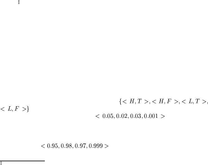
For example, consider the Cancer node of Figure 2.1. Its parents are Pollution

and Smoking and take the possible joint values

. The conditional probability table speciﬁes in order the probability of

cancer for each of these cases to be:

. Since these are

probabilities, and must sum to one over all possible states of the Cancer variable,

the probability of no cancer is already implicitly given as one minus the above prob-

abilities in each case; i.e., the probability of no cancer in the four possible parent

instantiations is

Oddly, this is the antipodean standard in computer science; we’ll let you decide what that may mean

about computer scientists!

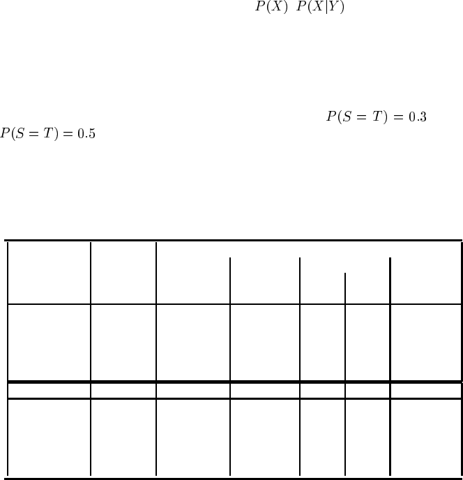
Root nodes also have an associated CPT, although it is degenerate, containing only

one row representing its prior probabilities. In our example, the prior for a patient

being a smoker is given as 0.3, indicating that 30% of the population that the doctor

sees are smokers, while 90% of the population are exposed to only low levels of

pollution.

Clearly, if a node has many parents or if the parents can take a large number of

values, the CPT can get very large! The size of the CPT is, in fact, exponential in the

number of parents. Thus, for Boolean networks a variable with

parents requires a

CPT with

probabilities.

2.2.4 The Markov property

In general, modeling with Bayesian networks requires the assumption of the Markov

property: there are no direct dependencies in the system being modeled which are

not already explicitly shown via arcs. In our Cancer case, for example, there is no

way for smoking to inﬂuence dyspnoea except by way of causing cancer (or not)

— there is no hidden “backdoor” from smoking to dyspnoea. Bayesian networks

which have the Markov property are also called Independence-maps (or, I-maps

for short), since every independence suggested by the lack of an arc is real in the

system.

Whereas the independencies suggested by a lack of arcs are generally required to

exist in the system being modeled, it is not generally required that the arcs in a BN

correspond to real dependencies in the system. The CPTs may be parameterized in

such a way as to nullify any dependence. Thus, for example, every fully-connected

Bayesian network can represent, perhaps in a wasteful fashion, any joint probability

distribution over the variables being modeled. Of course, we shall prefer minimal

models and, in particular, minimal I-maps, which are I-maps such that the deletion

of any arc violates I-mapness by implying a non-existent independence in the system.

If, in fact, every arc in a BN happens to correspond to a direct dependence in the

system, then the BN is said to be a Dependence-map (or, D-map for short). A BN

whichisbothanI-mapandaD-mapissaidtobeaperfect map.

2.3 Reasoning with Bayesian networks

Now that we know how a domain and its uncertainty may be represented in a Bayes-

ian network, we will look at how to use the Bayesian network to reason about the

domain. In particular, when we observe the value of some variable, we would like to

condition upon the new information. The process of conditioning (also called prob-

ability propagation or inference or belief updating) is performed via a “ﬂow of

information” through the network. Note that this information ﬂow is not limited to

the directions of the arcs. In our probabilistic system, this becomes the task of com-

puting the posterior probability distribution for a set of query nodes, given values

for some evidence (or observation) nodes.

2.3.1 Types of reasoning

Bayesian networks provide full representations of probability distributions over their

variables. That implies that they can be conditioned upon any subset of their vari-

ables, supporting any direction of reasoning.

For example, one can perform diagnostic reasoning, i.e., reasoning from symp-

toms to cause, such as when a doctor observes Dyspnoea and then updates his belief

about Cancer and whether the patient is a Smoker. Note that this reasoning occurs in

the opposite direction to the network arcs.

Or again, one can perform predictive reasoning, reasoning from new information

about causes to new beliefs about effects, following the directions of the network

arcs. For example, the patient may tell his physician that he is a smoker; even before

any symptoms have been assessed, the physician knows this will increase the chances

of the patient having cancer. It will also change the physician’s expectations that the

patient will exhibit other symptoms, such as shortness of breath or having a positive

X-ray result.

Query

direction of reasoning

Query

Evidence

Query

QueryQuery

Query

Evidence

EvidenceQuery

Evidence

(explaining away)

Evidence

COMBINED

PREDICTIVE

INTERCAUSAL

DIAGNOSTIC

FIGURE 2.2

Types of reasoning.

A further form of reasoning involves reasoning about the mutual causes of a com-

mon effect; this has been called intercausal reasoning. A particular type called

explaining away is of some interest. Suppose that there are exactly two possible

causes of a particular effect, represented by a v-structure in the BN. This situation

occurs in our model of Figure 2.1 with the causes Smoker and Pollution which have a

common effect, Cancer (of course, reality is more complex than our example!). Ini-

tially, according to the model, these two causes are independent of each other; that is,

a patient smoking (or not) does not change the probability of the patient being sub-

ject to pollution. Suppose, however, that we learn that Mr. Smith has cancer. This

will raise our probability for both possible causes of cancer, increasing the chances

both that he is a smoker and that he has been exposed to pollution. Suppose then that

we discover that he is a smoker. This new information explains the observed can-

cer, which in turn lowers the probability that he has been exposed to high levels of

pollution. So, even though the two causes are initially independent, with knowledge

of the effect the presence of one explanatory cause renders an alternative cause less

likely. In other words, the alternative cause has been explained away.

Since any nodes may be query nodes and any may be evidence nodes, sometimes

the reasoning does not ﬁt neatly into one of the types described above. Indeed, we

can combine the above types of reasoning in any way. Figure 2.2 shows the different

varieties of reasoning using the Cancer BN. Note that the last combination shows the

simultaneous use of diagnostic and predictive reasoning.

2.3.2 Types of evidence

So Bayesian networks can be used for calculating new beliefs when new information

– which we have been calling evidence – is available. In our examples to date, we

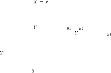
have considered evidence as a deﬁnite ﬁnding that a node X has a particular value,

x, which we write as

. This is sometimes referred to as speciﬁc evidence.

For example, suppose we discover the patient is a smoker, then Smoker=T,whichis

speciﬁc evidence.

However, sometimes evidence is available that is not so deﬁnite. The evidence

might be that a node

has the value or (implying that all other values are

impossible). Or the evidence might be that

is not in state (but may take any of

its other values); this is sometimes called a negative evidence.

In fact, the new information might simply be any new probability distribution

over

. Suppose, for example, that the radiologist who has taken and analyzed the

X-ray in our cancer example is uncertain. He thinks that the X-ray looks positive,

but is only 80% sure. Such information can be incorporated equivalently to Jeffrey

conditionalization of

1.5.1, in which case it would correspond to adopting a new

posterior distribution for the node in question. In Bayesian networks this is also

known as virtual evidence. Since it is handled via likelihood information, it is also

known as likelihood evidence. We defer further discussion of virtual evidence until

Chapter 3, where we can explain it through the effect on belief updating.

2.3.3 Reasoning with numbers

Now that we have described qualitatively the types of reasoning that are possible

using BNs, and types of evidence, let’s look at the actual numbers. Even before we

obtain any evidence, we can compute a prior belief for the value of each node; this

is the node’s prior probability distribution. We will use the notation Bel(X) for the

posterior probability distribution over a variable X, to distinguish it from the prior

and conditional probability distributions (i.e.,

, ).

The exact numbers for the updated beliefs for each of the reasoning cases de-

scribed above are given in Table 2.2. The ﬁrst set are for the priors and conditional

probabilities originally speciﬁed in Figure 2.1. The second set of numbers shows

what happens if the smoking rate in the population increases from 30% to 50%,

as represented by a change in the prior for the Smoker node. Note that, since the

two cases differ only in the prior probability of smoking (

versus

), when the evidence itself is about the patient being a smoker, then

the prior becomes irrelevant and both networks give the same numbers.

TABLE 2.2

Updated beliefs given new information with smoking rate 0.3 (top set) and 0.5

(bottom set)

Node No Reasoning Case

P(S)=0.3 Evidence Diagnostic Predictive Intercausal Combined

D=T S=T C=T C=T D=T

S=T S=T

Bel(P=high) 0.100 0.102 0.100 0.249 0.156 0.102

Bel(S=T) 0.300 0.307 1 0.825 1 1

Bel(C=T) 0.011 0.025 0.032 1 1 0.067

Bel(X=pos) 0.208 0.217 0.222 0.900 0.900 0.247

Bel(D=T) 0.304 1 0.311 0.650 0.650 1

P(S)=0.5

Bel(P=high) 0.100 0.102 0.100 0.201 0.156 0.102

Bel(S=T) 0.500 0.508 1 0.917 1 1

Bel(C=T) 0.174 0.037 0.032 1 1 0.067

Bel(X=pos) 0.212 0.226 0.311 0.900 0.900 0.247

Bel(D=T) 0.306 1 0.222 0.650 0.650 1

Belief updating can be done using a number of exact and approximate inference al-

gorithms. We give details of these algorithms in Chapter 3, with particular emphasis

on how choosing different algorithms can affect the efﬁciency of both the knowledge

engineering process and the automated reasoning in the deployed system. However,

most existing BN software packages use essentially the same algorithm and it is quite

possible to build and use BNs without knowing the details of the belief updating al-

gorithms.

2.4 Understanding Bayesian networks

We now consider how to interpret the information encoded in a BN — the proba-

bilistic semantics of Bayesian networks.

2.4.1 Representing the joint probability distribution

Most commonly, BNs are considered to be representations of joint probability distri-

butions. There is a fundamental assumption that there is a useful underlying struc-

ture to the problem being modeled that can be captured with a BN, i.e., that not every

node is connected to every other node. If such domain structure exists, a BN gives

a more compact representation than simply describing the probability of every joint

instantiation of all variables. Sparse Bayesian networks (those with relatively few

arcs, which means few parents for each node) represent probability distributions in a

computationally tractable way.

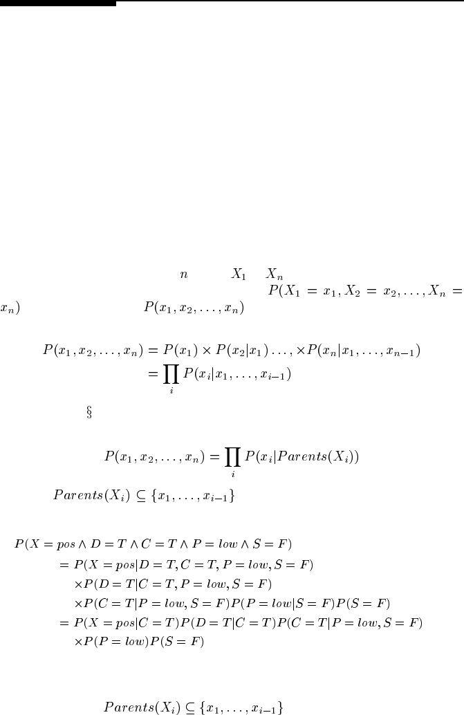
Consider a BN containing the

nodes, to , taken in that order. A particular

value in the joint distribution is represented by

, or more compactly, .Thechain rule of probability theory

allows us to factorize joint probabilities so:

(2.1)

Recalling from

2.2.4 that the structure of a BN implies that the value of a particular

node is conditional only on the values of its parent nodes, this reduces to

provided . For example, by examining Figure 2.1,

we can simplify its joint probability expressions. E.g.,

2.4.2 Pearl’s network construction algorithm

The condition that allows us to construct a network

from a given ordering of nodes using Pearl’s network construction algorithm [217,

section 3.3]. Furthermore, the resultant network will be a unique minimal I-map,

assuming the probability distribution is positive. The construction algorithm (Algo-

rithm 2.1) simply processes each node in order, adding it to the existing network and

adding arcs from a minimal set of parents such that the parent set renders the current

node conditionally independent of every other node preceding it.

ALGORITHM 2.1

Pearl’s Network Construction Algorithm

1. Choose the set of relevant variables

that describe the domain.

2. Choose an ordering for the variables,

3. While there are variables left:

(a) Add the next variable

to the network.

(b) Add arcs to the

node from some minimal set of nodes already in the net,

, such that the following conditionalindependenceproperty

is satisﬁed:

where are all the variables preceding that are not in

2.4.3 Compactness and node ordering

Using this construction algorithm, it is clear that a different node order may result

in a different network structure, with both nevertheless representing the same joint

probability distribution.

In our example, several different orderings will give the original network structure:

Pollution and Smoker must be added ﬁrst, but in either order, then Cancer,andthen

Dyspnoea and X-ray, again in either order.

On the other hand, if we add the symptoms ﬁrst, we will get a markedly different

network. Consider the order

. D is now the new root node.

When adding X, we must consider “Is X-ray independent of Dyspnoea?” Since they

have a common cause in Cancer, they will be dependent: learning the presence of

one symptom, for example, raises the probability of the other being present. Hence,

we have to add an arc from

to . When adding Cancer, we note that Cancer

is directly dependent upon both Dyspnoea and X-ray, so we must add arcs from

both. For Pollution, an arc is required from

to to carry the direct dependency.

When the ﬁnal node, Smoker, is added, not only is an arc required from

to ,

but another from

to . In our story and are independent, but in the new

network, without this ﬁnal arc,

and are made dependent by having a common

cause, so that effect must be counterbalanced by an additional arc. The result is two

additional arcs and three new probability values associated with them, as shown in

Figure 2.3(a). Given the order

, we get Figure 2.3(b), which is

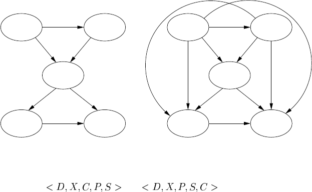
fully connected and requires as many CPT entries as a brute force speciﬁcation of

the full joint distribution! In such cases, the use of Bayesian networks offers no

representational, or computational, advantage.

(a)

(b)

Dyspnoea

XRay

Cancer

Smoker

Pollution

XRay

Cancer

Smoker

Pollution

FIGURE 2.3

Alternative structures obtained using Pearl’s network construction algorithm with

orderings: (a)

;(b) .

It is desirable to build the most compact BN possible, for three reasons. First,

the more compact the model, the more tractable it is. It will have fewer probability

values requiring speciﬁcation; it will occupy less computer memory; probability up-

dates will be more computationally efﬁcient. Second, overly dense networks fail to

represent independencies explicitly. And third, overly dense networks fail to repre-

sent the causal dependencies in the domain. We will discuss these last two points

just below.

We can see from the examples that the compactness of the BN depends on getting

the node ordering “right.” The optimal order is to add the root causes ﬁrst, then

the variable(s) they inﬂuence directly, and continue until leaves are reached. To

understand why, we need to consider the relation between probabilistic and causal

dependence.

2.4.4 Conditional independence

Bayesian networks which satisfy the Markov property (and so are I-maps) explic-

itly express conditional independencies in probability distributions. The relation

between conditional independence and Bayesian network structure is important for

understanding how BNs work.

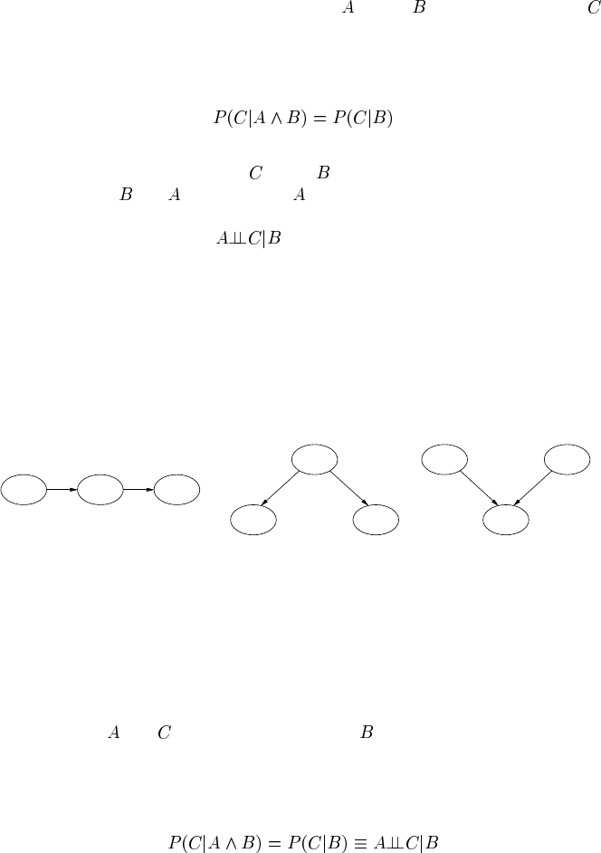
2.4.4.1 Causal chains

Consider a causal chain of three nodes, where

causes whichinturncauses ,

as shown in Figure 2.4(a). In our medical diagnosis example, one such causal chain

is “smoking causes cancer which causes dyspnoea.” Causal chains give rise to con-

ditional independence, such as for Figure 2.4(a):

This means that the probability of ,given , is exactly the same as the probability

of C, given both

and . Knowing that has occurred doesn’t make any difference

to our beliefs about C if we already know that B has occurred. We also write this

conditional independence as:

In Figure 2.1(a), the probability that someone has dyspnoea depends directly only

on whether they have cancer. If we don’t know whether some woman has cancer,

but we do ﬁnd out she is a smoker, that would increase our belief both that she has

cancer and that she suffers from shortness of breath. However, if we already knew

she had cancer, then her smoking wouldn’t make any difference to the probability of

dyspnoea. That is, dyspnoea is conditionally independent of being a smoker given

the patient has cancer.

(b) (c)

(a)

CBA

FIGURE 2.4

(a) Causal chain; (b) common cause; (c) common effect.

2.4.4.2 Common causes

Two variables

and having a common cause is represented in Figure 2.4(b).

In our example, cancer is a common cause of the two symptoms, a positive X-ray

result and dyspnoea. Common causes (or common ancestors) give rise to the same

conditional independence structure as chains:

If there is no evidence or information about cancer, then learning that one symptom is

present will increase the chances of cancer which in turn will increase the probability

of the other symptom. However, if we already know about cancer, then an additional

positive X-ray won’t tell us anything new about the chances of dyspnoea.

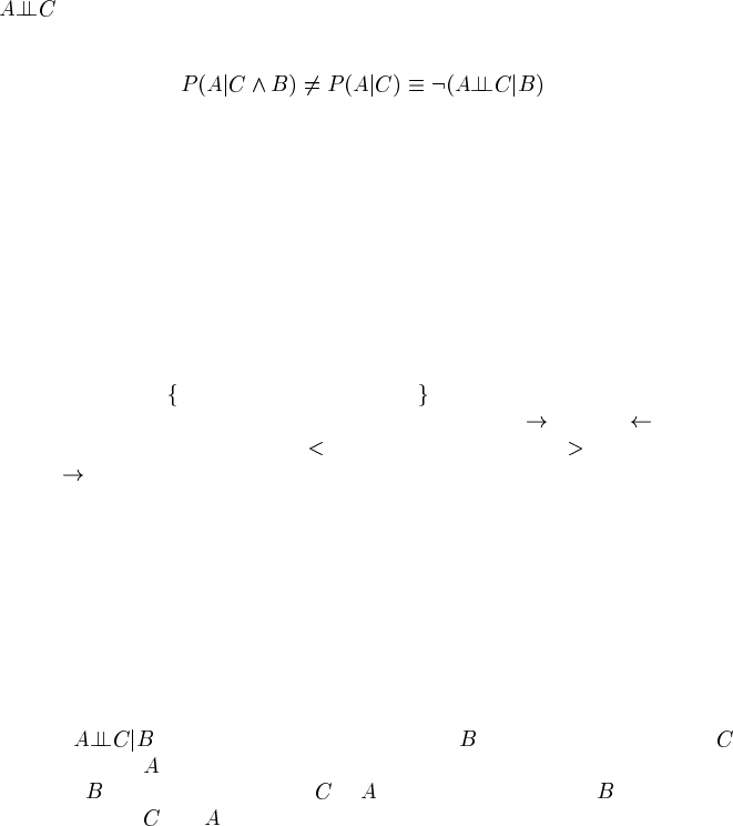
2.4.4.3 Common effects

A common effect is represented by a network v-structure, as in Figure 2.4(c). This

represents the situation where a node (the effect) has two causes. Common effects (or

their descendants) produce the exact opposite conditional independence structure to

that of chains and common causes. That is, the parents are marginally independent

(

), but become dependent given information about the common effect (i.e.,

they are conditionally dependent):

Thus, if we observe the effect (e.g., cancer), and then, say, we ﬁnd out that one of

the causes is absent (e.g., the patient does not smoke), this raises the probability of

the other cause (e.g., that he lives in a polluted area) — which is just the inverse of

explaining away.

Compactness again

So we can now see why building networks with an order violating causal order can,

and generally will, lead to additional complexity in the form of extra arcs. Consider

just the subnetwork

Pollution, Smoker, Cancer of Figure 2.1. If we build the sub-

network in that order we get the simple v-structure Pollution

Smoker Cancer.

However, if we build it in the order

Cancer, Pollution, Smoker , we will ﬁrst get

Cancer

Pollution, because they are dependent. When we add Smoker, it will be

dependent upon Cancer, because in reality there is a direct dependency there. But we

shall also have to add a spurious arc to Pollution, because otherwise Cancer will act

as a common cause, inducing a spurious dependency between Smoker and Pollution;

the extra arc is necessary to reestablish marginal independence between the two.

2.4.5 d-separation

We have seen how Bayesian networks represent conditional independencies and how

these independencies affect belief change during updating. The conditional indepen-

dence in

means that knowing the value of blocks information about

being relevant to , and vice versa. Or, in the case of Figure 2.4(c), lack of informa-

tion about

blocks the relevance of to , whereas learning about activates the

relation between

and .

These concepts apply not only between pairs of nodes, but also between sets of

nodes. More generally, given the Markov property, it is possible to determine whe-

ther a set of nodes X is independent of another set Y, given a set of evidence nodes

E. To do this, we introduce the notion of d-separation (from direction-dependent

separation).