Hou G.W.S. Flavor Physics and the TeV Scale

Подождите немного. Документ загружается.

72 4 H

Probes: b → s␥ and B → τν

23. Hou, W.S.: Phys. Rev. D 48, 2342 (1993) 65, 66, 70, 71

24. The paper only appeared in 1995, Artuso, M., et al. [CLEO Collaboration]: Phys. Rev. Lett.

75, 785 (1995) 65

25. Ikado, K., et al. [Belle Collaboration]: Phys. Rev. Lett. 97, 251802 (2006) 67, 68

26. Aubert, B., et al. [BaBar Collaboration]: Phys. Rev. D 77, 011107 (2008) 67, 68

27. Matyja, A., et al. [Belle Collaboration]: Phys. Rev. Lett. 99, 191807 (2007) 68

28. Aubert, B., et al. [BaBar Collaboration]: Phys. Rev. Lett. 100, 021801 (2008) 69

29. Grza¸dkowski, B., Hou, W.S.: Phys. Lett. B 283, 427 (1992) 69, 70

30. Artuso, M., et al. [CLEO Collaboration]: Phys. Rev. Lett. 99, 071802 (2007) 70

31. Widhalm, L., et al. [Belle Collaboration]: Phys. Rev. Lett. 100, 241801 (2008) 70

32. Aubert, B., et al. [BaBar Collaboration]: Phys. Rev. Lett. 98, 141801 (2007) 70

33. Dobrescu, B.A., Kronfeld, A.S., Phys. Rev. Lett. 100, 241802 (2008) 70, 71

34. Follana, E., Davies, C.T.H., Lepage, G.P., Shigemitsu, J., Phys. Rev. Lett. 100, 062002 (2008) 70

Chapter 5

Electroweak Penguin: bsZ Vertex, Z



Dark Matter

In Sect. 2.2, we discussed the effects of the b → s

qq electroweak penguin inter-

fering with the strong penguin and tree amplitudes. The quintessential electroweak

penguin would be b → s



−

decay or b → sνν that has no photonic contribution.

We now discuss how the study of these processes, present already in SM, could help

us probe New Physics as well. Besides presenting some background development,

we will focus on the forward–backward asymmetry A

(B → K

∗



−

) as a probe

of the bs Z vertex, comment brieﬂy on a possible Z



boson as a source for generating

effective [

sb][

] and [

sb][¯νν] four-fermi interactions, and treat b → sνν, which

has the same signature as b → s+ nothing, as a probe of light Dark Matter (DM).

5.1 A

(B → K

∗



−

)

5.1.1 Observation of m

Enhancement of b → s



−

The B → K

(∗)



−

process (b → s



−

at inclusive level) arises from photonic

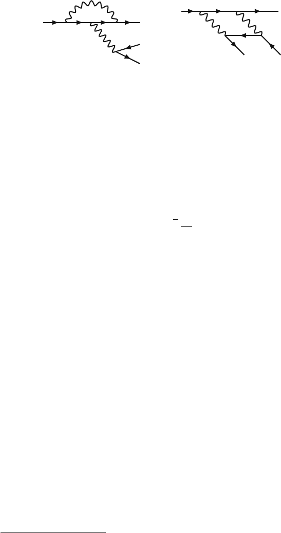
penguin, Z penguin, and box diagrams, as shown in Fig. 5.1.

At ﬁrst sight, one would think that the photonic penguin is at αG

order (α from

QED, G

from one W ), while the Z penguin and box diagrams, which have two

heavy vector boson propagators, are effectively at G

order of weak interactions.

Since G

is small compared to the physical decay scale of m

, it seems intuitive

to drop the Z penguin and box diagrams. This was in fact what was ﬁrst [1] done

historically. But it was soon pointed out [2] that the Z penguin (gauge related to

both the photon penguin and box diagrams) would in fact dominate for large m

We have already discussed this “nondecoupling” phenomenon of the SM heavy t

quark in Sect. 3.2.3, but it is worthwhile to understand the origins of this.

A heuristic way to see Z penguin dominance of b → s



−

is to observe that the

above “G

power counting” has a loophole. Comparing αG

of the photonic pen-

guin with G

of the Z penguin, the two factors actually have different mass dimen-

sions. To compensate, the latter should be written as G

. This has been used in

our simple power counting above, where we have used m

in a tacit way. However,

from subtleties of the diagrams involved, and supported by a full calculation, one

G.W.S. Hou, Flavor Physics and the TeV Scale, STMP 233, 73–86,

DOI 10.1007/978-3-540-92792-1



Springer-Verlag Berlin Heidelberg 2009

74 5 Electroweak Penguin: bsZ Ve rt ex, Z



, Dark Matter

γ,

, (¯ν)

−

, (ν)

, (¯ν)

−

, (ν)

−

Fig. 5.1 Photonic penguin, Z penguin, and the box diagram for b → s



−

, sν ¯ν

ﬁnds m

instead of m

as the outcome. G

is certainly not negligible compared

to α for m

above 100 GeV or so.

The source of this nondecoupling of SM heavy quarks is due to their large

Yukawa couplings. Note that heavy particle propagators in general lead to decou-

pling, i.e., heavy mass effects are normally decoupled, with G

power counting as

a good example.

So, one would have thought that the effect of a heavy top would

also be decoupled. In pure QED and QCD processes, this would indeed be the case.

However, the weak interaction (or SU(2)×U(1)) is more complicated:

≡

√

(5.1)

is the dynamical Yukawa coupling, where v is the v.e.v. scale. The heaviness of m

is a dynamical effect. It turns out that two powers of Yukawa couplings remain for

the Z loop calculation, which results in nondecoupling. So why does this not happen

for the photonic penguin?

It is not our purpose to present any diagrammatic calculations. However, it would

be elucidating to give an account of the subtleties that distinguishes the ␥ and Z

penguins, i.e.,

sb␥ and

sbZ couplings. So let us try to be as lucid as possible

and explain in a language that hopefully even experimenters can grasp (see also

Footnote 3 of Chap. 4). In attempting the calculations for the diagrams of Fig. 5.1,

one would like to ignore all external masses and momenta as much as possible, since

is small (i.e., G

is negligible). In so doing, one then discovers that the

sb␥ vertex would vanish in the m

→ 0 limit. Hence, to extract the

sb␥ vertex,

extra care needs to be taken, and one needs to make an expansion in small external

masses and momenta, before setting them to zero. Alternatively, one recalls that the

photon, even if off-shell, couples to conserved currents. This is a requirement of

gauge invariance. A vanishing vertex is of course trivially conserved, but to have a

nontrivially conserved

sb␥ vertex, the effective vertex would depend on the external

momentum and mass(es). The point is that m

and m

are of unequal mass, so

s␥

is not a conserved current.

In the notation of Inami and Lim [3], we write the effective

sb␥ vertex as



␥

−q

q/) F

+iσ

μν

R + m

L) F



b, (5.2)

Technically, this statement is actually not true. For low energy tree-level effects, it is the process

mass scale vs M

scale that provides suppression. See below.

5.1 A

(B → K

∗



−

)75

where q is the four-momentum carried off by the photon. It is clear that (5.2) is

explicitly conserved, i.e., contracting with q

, both terms vanish. Note that the q

term, when contracting with another conserved current (e.g.,

␥

 in our case, or an

external photon polarization vector), would vanish. Furthermore, the contribution of

the F

“form factor” would vanish for on-shell (q

= 0) photons. So, it is the F

term that contributes to physical b → s␥ decay, but both F

and F

contribute to

b → s



−

We see now what must be collected in expanding the

sb␥ vertex of Fig. 5.1: we

must collect q

␥

and q

,aswellasσ

μν

b,s

terms. That they come together to

give the form of (5.2) is a check on the calculation. In contrast, the

sbZ vertex is not

conserved, because the electroweak gauge invariance is spontaneously broken down

to electromagnetism. Thus, in computing the

sbZ vertex of Fig. 5.1, one does not

need to put the vertex in the form of (5.2), and in fact one could set m

to zero

from the outset. It is this subtlety, that the electromagnetic current is conserved, but

the charge and neutral current is not, that sets apart the behavior (in m

dependence)

of the

sb␥ and

sbZ couplings.

The result above is of course gauge invariant. In the physical gauge, the longitudi-

nal components of the W

boson lead to m

in the numerator in the

tbW

coupling.

In gauges where one has unphysical scalars φ

, these are the would-be Goldstone

bosons that got “eaten” by the W

boson to make it heavy, and, as a partner to

the SM neutral Higgs boson, it couples to top via (5.1). The whole picture works

consistently for the

sbZ vertex, which is not conserved, but for the

sb␥ vertex, the

requirement of (5.2) by current conservation replaces the possible m

factors by q

and m

b(s)

q, and the m

effect for

sb␥ is closer to the decoupling kind,

as already

commented on in Sect. 3.2.3.

We have thus given arguments for why the m

dependence of photonic and Z

penguins are so different, and how the latter could dominate for large enough m

It is intricately related to spontaneous symmetry breaking and mass generation in

the electroweak theory. A full calculation of course bears all this out. We plot in

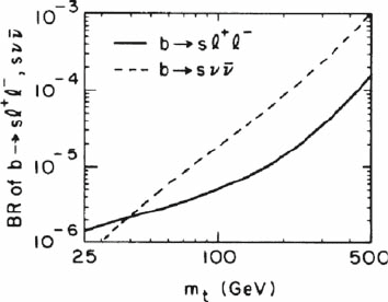
Fig. 5.2 the more than 20 years old result from the original observation [2] of large

enhancement of the decay rates of b → s



−

, sν ¯ν. Note that b → sμ

−

is slightly smaller than b → se

−

, because the latter has a low q

enhancement

from the photonic penguin. The strong, almost m

dependence is most apparent

for b → sν ¯ν, which has no photon contribution, and we have summed over three

neutrinos. Of course, much progress has been made in sophisticated calculations of

the rates of b → s



−

, sν ¯ν. However, the results of Fig. 5.2 captures the main

effect, and all subsequent calculations are corrections.

Although b → s␥ was already observed by CLEO in the 1990s, the ﬁrst observa-

tion of an electroweak penguin decay was only made by Belle in 2001. With 31.3M

B pairs, combining B → Ke

−

and K μ

−

events (K stands for both charged

and neutral kaons), Belle observed [4] ∼14 events with a combined statistical

For the

sb␥ vertex, the photon can also radiate off the W

(not shown in Fig. 5.1). But for the

sbg vertex, the gluon can only radiate off the top. With always two top propagators, the

sbg vertex

has even weaker m

dependence.

76 5 Electroweak Penguin: bsZ Ve rt ex, Z



, Dark Matter

Fig. 5.2 Large m

enhancement [2] of b → s



−

, sν ¯ν rates. [Copyright (1987) by The American

Physical Society.]

signiﬁcance of 5.3σ for B → K 



−

. The result was consistent with SM, but

subject to B → K form factors, so the interpretation is less interesting. Observation

of B → K

∗



−

[5, 6] soon followed. Repeating the b → s␥ history, the inclu-

sive b → s



−

measurement (B → X



−

experimentally) was subsequently

observed a year or so later, by Belle in summer 2002. With 65.4M B

B pairs and

again combining e

−

and μ

−

, a total of ∼60 events were observed [7] with

5.4σ statistical signiﬁcance, and b → s



−

became experimentally established.

Many modes, including the exclusive B → π, ρ modes (replacing s by d

in Fig. 5.2), have now been searched for. A new study, based on 657M B

B pairs by

Belle [8], has pushed the limit on B

→ π



−

down to the 5×10

−8

level, which

is only a factor of 1.5 above SM expectations [9]. Put differently, it seems that the

measurement of B → π and b → d is a Super B Factory subject.

In the experimental studies, one cuts out the J/ψ and ψ



resonance regions

in q

, as these produce the same ﬁnal states and are in fact much larger. These

charmonium regions actually provide a large control sample to test the ﬁt models

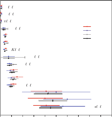
for the electroweak penguin study. The results on electroweak penguins as of 2008

are summarized in Fig. 5.3. The inclusive rate is consistent with SM expectations

(see, e.g., [10]), hence conﬁrming the large m

enhancement [2]. Note that the latter

observation was made in 1986, prior to the ARGUS discovery [11] of large B

mixing, which led to the change in mindset that the top quark is uniquely heavy.

Given that the top is a v.e.v. scale fermion, we could say that TeV scale physics

inﬂuenced the b → s rate, as a prime example of the ﬂavor–TeV link. Since

electroweak symmetry breaking is the main theme for the LHC as a machine to

probe, to go above the v.e.v. scale, the complementary nature of b → s with

the high energy approach again resonates with the cartoon of Fig. 1.1. Our special

interest in the fourth generation can also be seen from this perspective [2]. The t



quark, being a SM-type chiral quark with mass generated through the analog of (5.1)

can also affect the bsZ coupling, so b → s is also a sensitive probe of t



,aswe

shall soon see.

5.1 A

(B → K

∗



−

)77

0.0 5.0 10.0

PDG2006

BABAR

Belle

New Avg.

HFAG

April 2008

Branching Ratio x 10

B(B

→



–

)

+ −

−

sμ

−

∗ + −

∗

−

∗

−

∗0 + −

∗+ + −

+ −

−

Kμ

−

0 + −

+ −

+ + −

0 + −

Fig. 5.3 HFAG plot for various B → X



−

measurements

5.1.2 B Factory Measurements of A

(B → K

∗



−

)

The top quark exhibits nondecoupling in the Z penguin and box diagrams, which is

analogous to the electroweak penguin effect in B

→ K

and the box diagrams

for B

–

mixing. We have elucidated that, due to this nondecoupling effect of the

top quark, the Z penguin dominates the b → s



−

decay amplitude [2].

Not long after the large m

enhancement was pointed out, it was soon noted

that interference between the vector (␥ and Z) and axial vector (Z only, box as

an appendage) contributions in b → s



−

production gives rise to an interesting

forward–backward asymmetry [12]. This is akin to the familiar A

in e

−

→ f

f ,

but the enhancement of the bs Z effective coupling compared with the bs␥ effective

coupling brings the Z from M

down to below the B mass, much closer to the ␥.

Furthermore, one now probes potential New Physics in the b → s loop. Since inter-

ference between amplitudes is the essence of quantum physics, thus, A

is of great

interest. In particular, for the differential dA

)/dq

asymmetry, the variation

over q

≡ m



probes different regions of interference between bs␥ and bsZ.

It is more than a ﬁgure of speech to say that the 



−

pair in the ﬁnal state, much

like an electron microscope that scatters an electron wave off the material being

probed, actually provides us with a “microscope” to look back at what is happening

inside the loop-induced bs␥ and bsZ vertices.

78 5 Electroweak Penguin: bsZ Ve rt ex, Z



, Dark Matter

With both the inclusive B → X



−

and exclusive B → K

(∗)



−

decays mea-

sured [5, 6, 13] (see Fig. 5.3), experimental interest turned to A

for B → K

∗



−

The study for inclusive A

, though desirable, is more challenging because of back-

ground issues and largely impossible in a hadronic environment. The experimentally

deﬁned forward–backward asymmetry is

)

≡

dB/dq

−dB/dq

−

dB/dq

+dB/dq

−

, (5.3)

where dB/dq

is the differential rate, and the ± superscript indicates forward and

backward moving 

versus the B meson direction in the 



−

frame.

Since the process is quite easy to visualize, let us give the quark level decay

amplitude [9],

b→s



−

∝ V

∗



− 2

eff

[

siσ

μν

Rb][

␥

]

eff

[

s␥

Lb][

␥

] +C

[

s␥

Lb][

␥

␥

]



, (5.4)

which is of the same form as 20 years ago [2], with short distance physics, includ-

ing within SM, isolated in the Wilson coefﬁcients C

eff

, C

eff

, and C

, which can be

systematically computed. The 1/q

term clearly carries the C

effective photon con-

tribution, which comes from the σ

μν

term in (5.2), while C

eff

and C

are from the Z

penguin (as well as the q

␥

term of (5.2) and the box diagram). We have factored

out V

∗

instead of the usual V

∗

. This has the advantage of being the product

of CKM elements that are already measured and real by standard convention [5, 6].

A commonly used formula for the differential A

)

∝ C

ξ(q

)



Re(C

eff

) F

eff



. (5.5)

The formulas for ξ (q

) and the form factor-related functions F

and F

can be found

in [9]. Within SM, the Wilson coefﬁcients are practically real, as has been ingrained

into the formula. This form has somehow inﬂuenced the development of the subject,

as we will discuss. Actually, C

eff

receives some long distance c

c effect that can be

absorptive [2], hence the real part is taken since this is not a CPV observable.

As shown in Fig. 5.4, the study of forward–backward asymmetry in B →

∗



−

by Belle with 386M B

B pairs [14] is consistent with SM and rules out

the possibility of ﬂipping the sign of C

or C

separately from SM value (the two

lower curves). But having both C

or C

ﬂipped in sign, equivalent to ﬂipping sign

of C

, is not ruled out. BaBar took the more conservative approach of giving A

in just two q

bins, below and above m

J/ψ

. With 229M B

B, the higher q

bin is

consistent [15] with SM and disfavors BSM scenarios. Interestingly, in the lower q

5.1 A

(B → K

∗



−

)79

–1

–0.5

0.5

4 6 8 10 12 14 16

18 20

(bkg-sub)

GeV

0 2 4 6 8 10 12 14 16 18 20

–0.4

–0.2

0.2

0.4

0.6

0.8

1.2

(2S)

Fig. 5.4 Measurements of A

(B → K

∗



−

Physical Society] and BaBar [16]. The two lower curves are for ﬂipping the sign of either C

with respect to SM (solid curve), while the upper curve is for C

and C

both ﬂipping sign

bin, while sign-ﬂipped BSMs are less favored, the measurement is ∼2σ away from

SM. This is not inconsistent with the Belle result.

BaBar has updated with 384M B

B pairs [16], which is shown in the second plot

in Fig. 5.4. For the high q

bin, the results are qualitatively the same as before. For

the low q

bin (4m

to 6.25 GeV

), BaBar has improved its measurement to

low q

= 0.24

+0.18

−0.23

± 0.05. The SM expectation in this region is A

low q

−0.03 ±0.01. Though not excluded, viewed together with the Belle result, it seems

that the low q

behavior is not quite SM-like.

5.1.3 Interpretation and Future Prospects

While the above is interesting, it should be clear that the B Factory statistics is still

rather limited and cannot be much improved without a Super B Factory. But LHCb

can do very well in this regard within a couple of years of LHC turn-on.

Note added: Belle announced their 657M B

B pair result at ICHEP2008 [17], improving on the

published result. All q

bins (six in all) turn out positive, and the deviation from SM becomes even

more acute. It would be desirable to give a combined experimental signiﬁcance on the deviation

from SM expectations.

80 5 Electroweak Penguin: bsZ Ve rt ex, Z



, Dark Matter

Wilson Coefﬁcients with Finite Weak Phase

In view of the LHCb prospects, we recently noticed [18] that, in (5.5), there is no

reason a priori why the Wilson coefﬁcients should be kept real when probing BSM

physics! This can be seen most easily by inspection of (5.4): the Wilson coefﬁcients

are effective couplings of four-fermi interactions, and in a theory that allows for

CPV, in general they should be complex from CPV phases. If one keeps an open

mind (rather than, for example, taking the oftentimes tacitly assumed Minimal Fla-

vor Violation, or MFV [19], mindset), (5.5) should be restored to its proper form,

)

∝ Re



eff

∗







eff

∗





, (5.6)

where we have absorbed ξ (q

) into the F



form factor combinations. In pointing

this out, we stress that we are not concerned with CP conserving long distance

effects such as in C

eff

, but the possibility that the C

s may pick up BSM weak (CP

violating) phases. If present, they could enrich the interference pattern through (5.6),

in contrast to the usual form of (5.5), which basically takes the short distance Wilson

coefﬁcients as real by ﬁat. After all, if P

is the culprit for the ⌬A

Kπ

problem

discussed in Sect. 2.2, the equivalent C

and C

for B

→ K

decay seem to

carry large weak phases. Let Nature speak through B → K

∗



−

data !

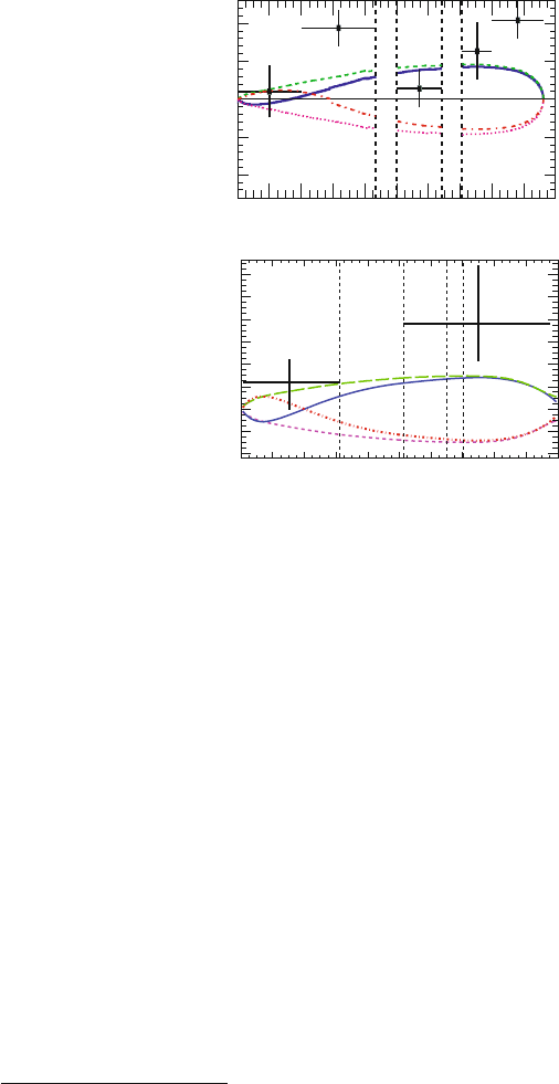
Taking the sign convention of LHCb, which is opposite to Belle and BaBar, we

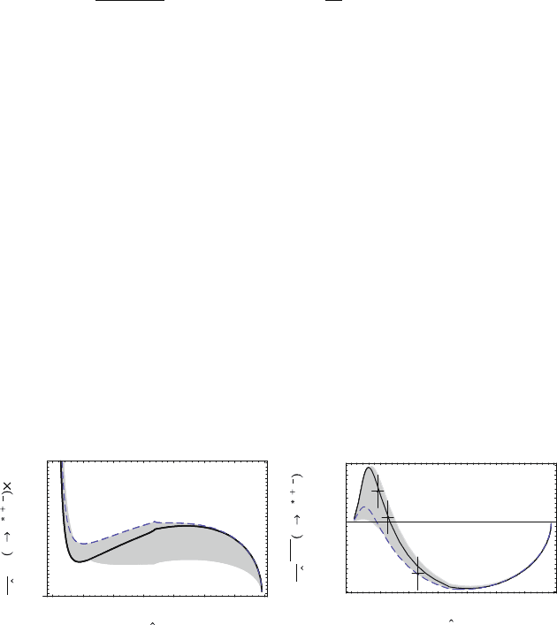
illustrate [18] in Fig. 5.5 the situation where New Physics enters through effec-

tive bsZ and bs␥ couplings. In this case, with 



−

produced from the virtual Z

∗

, and C

cannot differ by much at short distance, which is the reason for the

“degenerate tail” for larger

s ≡ q

(when the effect of C

becomes unimpor-

tant) in the dA

s plot. We allow the Wilson coefﬁcients to be only constrained

by the measured radiative (b → s␥) and electroweak (b → s) penguin rates,

hence dB/d

s may vary in the shaded area in Fig. 5.5, then dA

/dq

could in fact

vary in the corresponding shaded region, where the variation is more prominent

for q

< m

J/ψ

. Conventional wisdom suggest that it is the precise position of the

0 0.1 0.2 0.3 0.4 0.5 0.6 0.7

0.5

1.5

2.5

BR B K l l 10

0 0.1 0.2 0.3 0.4 0.5 0.6 0.7

–0.3

–0.2

–0.1

0.1

0.2

B K l l

Fig. 5.5 Possible dA

/dq

in B → K

∗



−

allowed by complex Wilson coefﬁcients [18], (5.6)

[Copyright (2008) by The American Physical Society]. The three data points are taken from 2 fb

−1

LHCb Monte Carlo for illustration, which has the power to distinguish between SM (solid curve)

vs e.g. fourth generation model (dashed curve). The sign convention is opposite that of Belle and

BaBar

5.1 A

(B → K

∗



−

)81

zero that is of interest, in part because it is less form factor dependent. We see that,

allowing for sizable weak phases for the Wilson coefﬁcients, the position of the zero

can be anywhere around or below the SM expectation.

The fourth generation with parameters as determined from ⌬m

, B(B →



−

) and ⌬A

Kπ

belongs to the class of BSM models of Fig. 5.5 and gives rise

to [18] the dashed line, which is close to the lower boundary of the shaded region for

s. The SM result is close to the upper boundary. Note that for the differential

decay rate, the fourth generation is at the upper boundary and could run into trouble

if the measured rate drops further. However, this would be a form factor-dependent

issue. To get a feeling for the future, we take the MC study [20, 21] for 2 fb

−1

data

by LHCb (achievable in a couple years of running, once LHC reaches productive

luminosity) and plot three sample data points for dA

s to illustrate expected

data quality. These data points are based on MC studies of events generated from

the SM (solid line). It is clear that LHCb can distinguish between SM and the fourth

generation, or other New Physics models in the shaded region.

Back to the present (closing) period of the B Factory era. From Fig. 5.5, we

could also compare with Belle and BaBar data [14–16] shown in Fig. 5.4 and see

that the current data are already probing the difference between SM and the fourth-

generation model

or the more general statement that Wilson coefﬁcients C

could

be complex, i.e., carry weak phase. As stated, the SM expectation is A

∼−0.03

(note the B Factory sign convention) for the region q

∈ (4m

,6.25GeV

This can be understood from the solid curve in Fig. 5.5(b), where the corresponding

region is

s < 0.22. Since there is a crossing over zero, and since the region below the

zero is slightly larger than above, we see that the SM expectation is slightly negative.

But Belle and BaBar data both indicate that A

> 0 is preferred. This is sometimes

phrased as “C

=−C

seems preferred from A

data,” but it should be viewed

as just a way of expression, since it has been pointed out [22] that C

=−C

, i.e.,

ﬂipping the sign of the photonic penguin, would lead to too large a B → X



−

rate as compared with experiment.

This actually illustrates our point to use (5.6) rather than (5.5) in ﬁtting data. In

fact, we could even claim that Belle and BaBar data favor somewhat the fourth-

generation curve in Fig. 5.5. Compared with the solid curve, the zero for the dashed

curve has moved to much lower q

, with a drop in peak value as well. Therefore, in

the fourth-generation model which is motivated by ⌬A

Kπ

(Sect. 2.2.2), and maybe

now the hint for large and negative sin 2⌽

as well (Sect. 3.2), we have A

> 0

for the low q

bin, which is in better agreement with data. This offers a third hint

that maybe the fourth-generation model where sizable b → s CPV phase should be

taken seriously !

It is gratifying that in their recent update, the BaBar experiment [16] has adopted our argument

and now uses (5.6) as the reference formula.