Hirsch M.J., Pardalos P.M., Murphey R. Dynamics of Information Systems: Theory and Applications

Подождите немного. Документ загружается.

216 M.A. Hurni et al.

numerous sources: Approximations in the modeling of the vehicle, errors in sensor

data, sensor accuracy, external unforeseen forces, and the error that is inherent in

executing the previous control solution while calculating an updated solution (the

lag between the two). The control interpolation error comes from the fact that low

node solutions are necessary to effect lower run times, which are required for real

time operation. A node is simply a discrete time point that describes the complete

vehicle state and control vectors at that speciﬁc time. If high number of nodes are

used, the trajectory can be made collision free, but at the expense of higher algorithm

run times. The proposed solution to this problem is the addition of the robustness

factor to a low-node problem deﬁnition. Since we desire to include robustness in

the cost function, it is necessary to derive a Robustness Function, r(t), whose in-

tegral over time will be minimum when robustness is maximized. To derive r(t),

we take (11.4) (which has a value of zero when on the obstacle and increases as

you move away from the obstacle) and apply a double exponential operation on

it [6]. This is done for each obstacle and the result is summed. The resulting r(t)

with n equal to the number of obstacles is (11.5). In the case of a single obsta-

cle, r(t) = 14.15 at its center, r(t) = 1.72 on its edge, and r(t) will continue to

decrease exponentially to zero as the distance to the obstacle is increased. Equa-

tion (11.6) is the ﬁnal cost function expressed in terms of the endpoint cost (ﬁ-

nal time) and the running cost (integral of r(t)) with appropriate weighting factors

(ω

,ω

r(t) =



i=1



−h

(x(t),y(t))

−1



(11.5)



(.), u(.), t



= ω

+ω



r(t)dt (11.6)

More details of UGV modeling/kinematics, obstacle modeling, and the trajec-

tory planning framework can be found in [5]. For all scenarios in this work, the

UGV mission is to traverse from an initial start point and reach the target point

in minimum time, with maximum robustness, while avoiding both static and dy-

namic obstacles. This is achieved by deriving the control solution that carries out

the initial planning problem while minimizing a cost and satisfying dynamical

and environmental constraints based on the initial global knowledge of the area.

To overcome the problem of incomplete global knowledge and a dynamic envi-

ronment, the UGV uses its sensors to map the locally detected changes in the

environment and continuously updates its global map; then recomputes and up-

dates the optimal trajectory at each information update [5]. The numerical solver

used to compute the optimal trajectories is the DIDO software package [10],

which is a MATLAB based software package that utilizes pseudospectral meth-

ods to determine an extremal for a properly formulated optimal control prob-

lem.

11 An Info-Centric Trajectory Planner for Unmanned Ground Vehicles 217

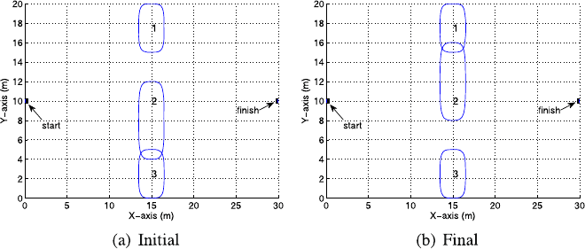
Fig. 11.1 Conﬁguration for sliding door problem

11.3 Obstacle Motion Studies

11.3.1 The Sliding Door

We start with the sliding door scenario of Figs. 11.1(a) and 11.1(b), which show the

initial and ﬁnal conﬁgurations of the environment obstacle, respectively. The start

and ﬁnish positions of the vehicle are as shown. All obstacles and the vehicle are

initially at rest. At 3 seconds into the maneuver, obstacle 2 moves north at a speed of

0.5 m/sec, gradually blocking the north passage and opening up the south passage.

The ﬁrst simulation was completed using snapshots of the environment taken

just prior to each iteration of the algorithm, with no prediction of obstacle position.

Thus, during the time it takes to generate a new solution, the vehicle maneuvers

based on the previous solution with no knowledge of obstacle motion until the next

snapshot is taken and the vehicle “senses” the environment has changed. Each run

produces a trajectory that solves the instantaneous static problem, even though the

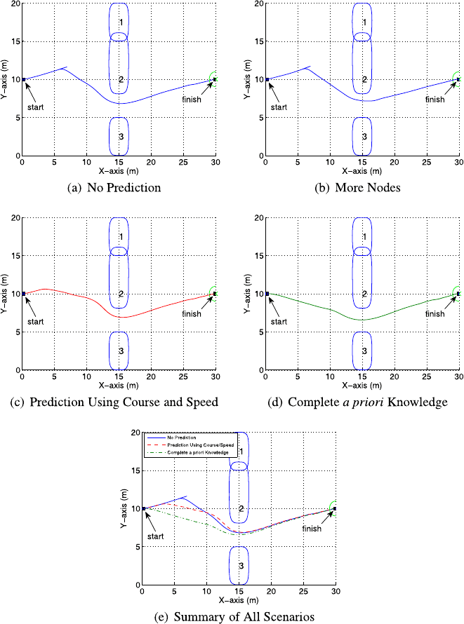
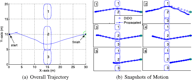
environment is dynamic. The resulting trajectory is shown in Fig. 11.2(a). The ve-

hicle heads toward the north passage until it is closed off, at which point the vehicle

stops, repositions (as required by the algorithm), generates a new bias, and then con-

tinues along the new path through the south passage. The trajectory in this case is

not perfectly smooth, which can be attributed to the fact that a low node PS-solution

results in higher propagation error. Figure 11.2b shows the smooth trajectory that

could be achieved with higher node solutions. Less smooth trajectories are accept-

able in trying to keep the number of nodes (and thus the run times) to a minimum.

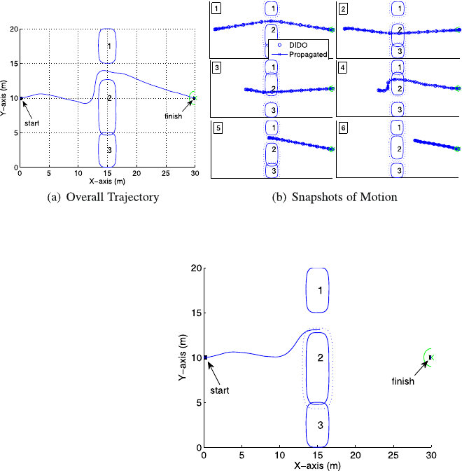
The sliding door scenario was repeated with the addition of obstacle position

prediction using course and speed. This can be achieved simply by comparing suc-

cessive environment snapshots to estimate a moving obstacle’s course and speed,

and then using that course and speed to predict the obstacle’s future position as part

of the trajectory planning problem. Figure 11.2(c) shows the resulting trajectory.

The vehicle initially heads toward the northern passage. Once obstacle 2 begins to

move north, the algorithm determines the obstacle’s future position using its course

218 M.A. Hurni et al.

Fig. 11.2 Various scenarios for sliding door problem

and speed, resulting in the vehicle autonomously changing its course to steer clear

of the obstacle. Obstacle 2 then stops moving, resulting in the vehicle making a new

course correction further to the south in order to steer clear. This course correction is

necessary because while the obstacle was moving, the prediction of its position was

11 An Info-Centric Trajectory Planner for Unmanned Ground Vehicles 219

based on the assumption that it would continue on its current course and speed. The

trajectory planner generates each new trajectory based on the current information

on obstacle positions, courses and speeds. It does not attempt to predict course or

speed changes. Any changes in the obstacle’s course and speed (including complete

stoppage) will require the planner to correct the vehicle’s trajectory accordingly.

Finally, the sliding door scenario was repeated with complete a priori knowl-

edge of obstacle 2 motion; i.e., all future course and speed changes of the obstacle

are known in advance. Figure 11.2(d) shows the resulting trajectory. The vehicle,

having complete knowledge of the future movement of obstacle 2, simply heads

immediately down the optimal path through the south passage.

The three sliding door scenarios with various levels of information are plotted to-

gether on Fig. 11.2(e). The scenarios using no prediction and using course and speed

for prediction start on the same trajectory, because obstacle 2 does not start moving

until the three-second point into the simulations. Without obstacle motion, the two

scenarios are identical. Once obstacle motion begins, using prediction results in a

trajectory that is closer to the time-optimal solution based on complete a priori in-

formation. When the obstacle position is not predicted, the maneuver time is 41.3

seconds, which does not include the extra time it takes to calculate a new southerly

bias when the north passage becomes blocked. When prediction is used, the maneu-

ver time is 33.5 seconds. With complete a priori knowledge of the environment, the

maneuver time is even shorter at 33 seconds.

11.3.2 The Cyclic Sliding Door

The sliding door scenario is modiﬁed so that the door continuously slides back and

forth, thus alternately blocking the north and south passages. This type of prob-

lem provides the opportunity to examine the trajectory planning algorithm’s per-

formance at all three information levels (i.e., no prediction, prediction, and a priori

knowledge). It allows us to simulate success or failure in algorithm performance

by simply adjusting the cycling speed of obstacle 2 (i.e., raising and lowering its

cycling frequency). It should be noted at the outset that given the maximum vehicle

speed of 1 m/sec and the obstacle widths of 3 m (not including their expansion to

account for vehicle size, see [5]), any obstacle 2 speed greater than 0.6 m/sec will

result in failure, because the vehicle cannot traverse through the opening quickly

enough. In other words, above a cycling speed of 0.6 m/sec there can be no solution

to the problem due to the physical limit on the vehicle speed.

We start at the lowest information level (i.e., no prediction using course and

speed) and the slowest cycling speed for obstacle 2 set at 0.1 m/sec. In this scenario,

obstacle 2 moves so slowly that it never has a chance to reverse course and head

south before the end of the vehicle’s mission. In other words, it doesn’t even com-

plete a half cycle. The resulting trajectory is shown in Fig. 11.3(a). The position of

obstacle 2 in Fig. 11.3(a) corresponds to its ﬁnal position at the end of the scenario,

and does not indicate its position at the time the vehicle passed through the north

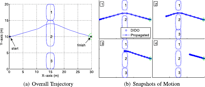
220 M.A. Hurni et al.

Fig. 11.3 Cyclic sliding door (no prediction; 0.1 m/sec cycle speed)

passage. Figure 11.3(b) shows the evolution of the trajectory at 4 sample instances

in time, and is composed of both the DIDO generated trajectory (circles correspond-

ing to discrete nodes) and the propagated path. The propagated path is obtained by

taking DIDO’s discrete control solution, applying control trajectory interpolation,

and then propagating the state trajectory using a Runge–Kutta algorithm. The fact

that the propagated and DIDO solutions fall on top of each other is the proof of

dynamic feasibility of the control solution. Obstacle 2’s movement is slow enough

that the vehicle need not change course to traverse the passage. The maneuver time

for this scenario was 33.5 seconds. Future ﬁgures showing the full vehicle trajec-

tory from start to ﬁnish will indicate obstacle positions at the ﬁnal time only (as in

Fig. 11.3(a)). Snapshots in time (as in Fig. 11.3(b)) will be given where appropriate.

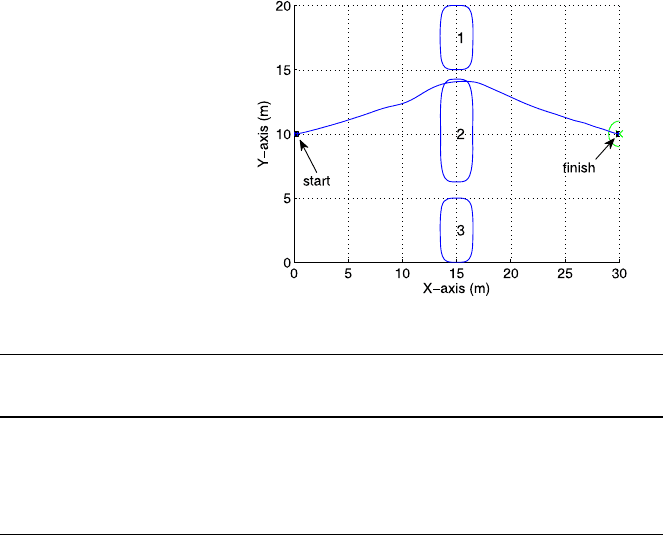
The cycle speed of the sliding door was then raised to 0.2 m/sec, which prevented

the vehicle from reaching the north passage in time to pass through. Since predic-

tion is not being used, the vehicle does not know the north passage will be closed

off until it actually happens. When the vehicle senses that the passage is blocked, it

stops, repositions, and reformulates a new bias. Figure 11.4 shows the resulting col-

lision (the dotted lines are the obstacle boundaries adjusted for the vehicle size). The

obstacle is moving slow enough to infer a solution exists, but, without prediction,

the vehicle cannot pass. The algorithm with this level of information also failed to

safely guide the vehicle through the passage (north or south) for all other speeds up

to the 0.6 m/sec limit. Sufﬁce it to say that without more information the algorithm

cannot safely guide the vehicle through this cyclic sliding door example.

The same scenarios presented above in Figs. 11.3(a) and 11.4 were simulated

again using obstacle position predicted from course and speed data. Figure 11.5(a)

shows the trajectory when the cycle speed is set to 0.1 m/sec. The maneuver time

was 33.4 seconds. The obstacle speed is too slow to show any signiﬁcant improve-

ment of the trajectory over the case of not utilizing current course and speed data to

calculate and include future obstacle positions while planning the vehicle’s trajec-

tory. The signiﬁcance of again showing the evolution of the trajectory (Fig. 11.5(b))

is in the change of the trajectory in the second frame of the ﬁgure. We see the tra-

jectory jump further away from the obstacle in frame 2, because the algorithm is

11 An Info-Centric Trajectory Planner for Unmanned Ground Vehicles 221

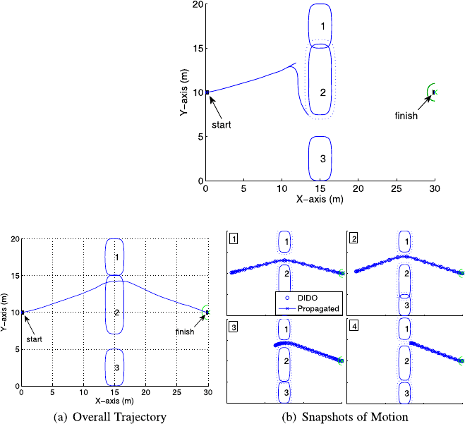
Fig. 11.4 Cyclic sliding door

(no prediction; 0.2 m/sec

cycle speed)

Fig. 11.5 Cyclic sliding door (with prediction; 0.1 m/sec cycle speed)

predicting the position of obstacle 2 as being further north at the time when the

vehicle traverses the north passage.

The cycle speed was again raised to 0.2 m/sec to show that with the addition of

prediction using course and speed, what was previously a trajectory planning fail-

ure became a success, as shown in Fig. 11.6(a). The vehicle initially heads to the

north passage. Once obstacle 2 begins moving, the algorithm predicts an infeasibil-

ity, because the intercept time of the vehicle with either passage results in complete

blockage of both passages (obstacle 2, when expanded to account for vehicle size,

completely blocks the path). The result is the vehicle stops, repositions, and refor-

mulates a new bias. In the time it takes the vehicle to stop and reposition, the inter-

cept time changes, and a solution then exists to allow the new bias to be generated

through the south passage. The total maneuver time in this case was 40 seconds.

The reason for the large increase in maneuver time is the fact that the vehicle stops

and repositions. It is obvious that rather than stop and reposition, the vehicle could

simply change its speed slightly to affect a different intercept time that would result

in an open south passage; however, it is counter to the minimum time formulation

of the optimal control problem to slow down (use less control effort) in order to

222 M.A. Hurni et al.

Fig. 11.6 Cyclic sliding door (with prediction; 0.2 m/sec cycle speed)

achieve a feasible path; therefore, its output indicates an infeasible trajectory us-

ing the maximum control effort. Figure 11.6(b) shows the evolution of the vehicle

trajectory. Notice the infeasibility in frame 2 of said ﬁgure.

The speed of obstacle 2 was further raised in 0.1 m/sec increments to determine

where the algorithm would fail when course and speed is used to predict obstacle

position. Figure 11.7(a) represents the trajectory corresponding to the fastest cycling

speed (0.5 m/sec) that the algorithm could handle. The total maneuver time was 36.3

seconds, which was faster than the case in Fig. 11.6(a), because the vehicle did not

have to stop and reposition. Figure 11.7(b) represents the evolution of the vehicle

trajectory. Frame 1 shows the trajectory prior to the commencement of obstacle 2

movement. In frames 2 and 3, obstacle 2 is moving north, resulting in the prediction

that the trajectory could wrap around the south side of the obstacle as it travels north.

In frames 4 and 5, obstacle 2 has changed directions to head south, which results

in a spontaneous replanning of the vehicle trajectory to wrap around the north side

of the obstacle. In frame 6, obstacle 2 has changed directions again and is headed

north, but by that point the vehicle has already safely navigated the north passage.

Clearly, if the algorithm can predict obstacle position using course and speed, it is

more effective than simply using still snapshots of the environment.

The next logical step here is to show the failure of the algorithm when the speed

of obstacle 2 is raised to 0.6 m/sec. Figure 11.8 illustrates that trajectory, which

changes direction (by prediction using course and speed) as the direction of obstacle

motion changes, but the obstacle motion is too fast for this method to be successful,

resulting in collision.

Finally, the cyclic sliding door scenario was repeated for different cycle speeds,

but this time more information was known by the algorithm; speciﬁcally, the al-

gorithm was given complete a priori knowledge of the motion of obstacle 2. Not

only were the instantaneous course and speeds known, but all the future course and

speed changes were also known in advance. Knowing the exact future position of

obstacle 2 resulted in a trajectory that headed directly for the correct position that

gave the vehicle safe passage. No replanning was necessary. Maneuver times at all

11 An Info-Centric Trajectory Planner for Unmanned Ground Vehicles 223

Fig. 11.7 Cyclic sliding door (with prediction; 0.5 m/sec cycle speed)

Fig. 11.8 Cyclic sliding door

(with prediction; 0.6 m/sec

cycle speed)

cycle speeds were the fastest possible (33.4 seconds). Figure 11.9 shows the tra-

jectory for the cycle speed of 0.6 m/sec, above which there can be no solution to

the problem due to the physical limit on vehicle speed. It follows that with advance

knowledge of environmental changes, the algorithm will always generate feasible

and safe trajectories within the physical limits of the vehicle.

Table 11.1 shows a summary of the results of executing the cyclic sliding door

scenario at various cycle speeds up to the vehicle’s limit using the three different

levels of information known to the algorithm. As expected, being able to predict

obstacle positions resulted in a higher success rate and better maneuver time than

not using prediction; and having a priori knowledge of environmental conditions

produced even better results. However, knowing the future positions of obstacles

beyond predicting them from their current course and speed is highly unlikely. It’s

assumed in this work that if an obstacle’s course and speed changes can be known

in advance, then it is likely another vehicle being controlled by the same home base,

which falls under multi-vehicle trajectory planning. For this reason, further motion

224 M.A. Hurni et al.

Fig. 11.9 Cyclic sliding door

(a priori knowledge;

0.6 m/sec cycle speed)

Table 11.1 Summary of results for cyclic sliding door scenario

Cycle speed (m/sec) Maneuver time (sec) Maneuver time (sec) Maneuver time (sec)

No prediction With prediction a priori knowledge

0.1 33.5 33.4 33.4

0.2 collision 40 33.4

0.5 collision 36.3 33.4

0.6 collision collision 33.4

studies will be limited to the comparisons between using prediction based on course

and speed and not using prediction (i.e., still snapshots of the environment).

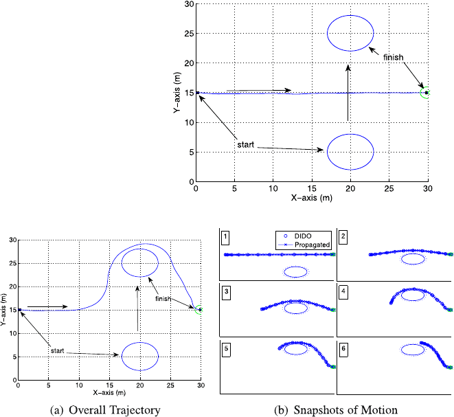
11.3.3 Obstacle Crossing (No Intercept)

This scenario can be described by any obstacle whose motion results in it cross-

ing over the trajectory of the vehicle, but does not pose a danger of collision. Fig-

ure 11.10 shows an example of the expected effect of a crossing obstacle on vehicle

trajectory. The obstacle starts out motionless, but after 5 seconds it moves from

(x, y =20, 5) meters to (x, y = 20, 25) meters at the speed of 1.5 m/sec across the

vehicle’s path as the vehicle travels from (x, y = 0, 15) meters to (x, y = 30, 15)

meters. The result shown in Fig. 11.10 was generated using course and speed to

predict the obstacle position. The overall maneuver time was 32.3 seconds.

If prediction is not used, the results are signiﬁcantly worse. The scenario of

Fig. 11.10 was repeated without prediction, and the resulting trajectory is shown in

Fig. 11.11(a) with a maneuver time that is signiﬁcantly higher at 49.9 seconds. Fig-

ure 11.11(b) shows the trajectory’s evolution over time. The ﬁgure shows that due to

the sensitivity of numerical optimization techniques (DIDO [10] in this case) to the

bias, the trajectory is pushed over the crossing obstacle, even though no collision

11 An Info-Centric Trajectory Planner for Unmanned Ground Vehicles 225

Fig. 11.10 Obstacle crossing

vehicle path (with prediction)

Fig. 11.11 Obstacle crossing vehicle path (no prediction)

course existed. The trajectory essentially gets shaped by any obstacles that cross its

path. The same effect can be produced by laying a string on a table whose endpoints

correspond to the desired start and goal positions, then sliding objects around the

table across the string, resulting in the string wrapping itself around those objects.

Adding prediction allows obstacles to skip over the string (trajectory) when encoun-

tered. Another situation that would allow for the obstacle to cross without adversely

affecting the trajectory is when the obstacle travels fast enough to cause it to skip

over the trajectory in successive environment snapshots.

11.3.4 Obstacle Intercept

The same obstacle crossing scenario was used, except the obstacle speed was

slowed down to 0.6 m/sec, which put it on a collision course with the vehicle.

Figure 11.12(a) shows the trajectory of the vehicle when using prediction, and the

maneuver time was 34.5 seconds. The time evolution of the trajectory is shown in