Greene W.H. Econometric Analysis

Подождите немного. Документ загружается.

CHAPTER 7

✦

Nonlinear, Semiparametric, Nonparametric Regression

189

A consistent estimator of σ

is based on the residuals:

ˆσ



i=1

− h(x

, b)]

. (7-16)

A degrees of freedom correction, 1/(n − K), where K is the number of elements in β,is

not strictly necessary here, because all results are asymptotic in any event. Davidson and

MacKinnon (2004) argue that on average, (7-16) will underestimate σ

, and one should

use the degrees of freedom correction. Most software in current use for this model does,

but analysts will want to verify which is the case for the program they are using. With

this in hand, the estimator of the asymptotic covariance matrix for the nonlinear least

squares estimator is given in (7-15).

Once the nonlinear least squares estimates are in hand, inference and hypothesis

tests can proceed in the same fashion as prescribed in Chapter 5. A minor problem can

arise in evaluating the ﬁt of the regression in that the familiar measure,

= 1 −



i=1



i=1

− ¯y)

, (7-17)

is no longer guaranteed to be in the range of 0 to 1. It does, however, provide a useful

descriptive measure.

7.2.4 HYPOTHESIS TESTING AND PARAMETRIC RESTRICTIONS

In most cases, the sorts of hypotheses one would test in this context will involve fairly

simple linear restrictions. The tests can be carried out using the familiar formulas dis-

cussed in Chapter 5 and the asymptotic covariance matrix presented earlier. For more

involved hypotheses and for nonlinear restrictions, the procedures are a bit less clear-

cut. Two principal testing procedures were discussed in Section 5.4: the Wald test, which

relies on the consistency and asymptotic normality of the estimator, and the F test, which

is appropriate in ﬁnite (all) samples, that relies on normally distributed disturbances.

In the nonlinear case, we rely on large-sample results, so the Wald statistic will be the

primary inference tool. An analog to the F statistic based on the ﬁt of the regression

will also be developed later. Finally, Lagrange multiplier tests for the general case can

be constructed. Since we have not assumed normality of the disturbances (yet), we

will postpone treatment of the likelihood ratio statistic until we revisit this model in

Chapter 14.

The hypothesis to be tested is

: r(β) = q, (7-18)

where r(β) is a column vector of J continuous functions of the elements of β. These

restrictions may be linear or nonlinear. It is necessary, however, that they be overiden-

tifying restrictions. Thus, in formal terms, if the original parameter vector has K free

elements, then the hypothesis r(β) −q must impose at least one functional relationship

on the parameters. If there is more than one restriction, then they must be functionally

independent. These two conditions imply that the J × K Jacobian,

R(β) =

∂r(β)

∂β



, (7-19)

190

PART I

✦

The Linear Regression Model

must have full row rank and that J , the number of restrictions, must be strictly less than

K. This situation is analogous to the linear model, in which R(β) would be the matrix of

coefﬁcients in the restrictions. (See, as well, Section 5.4, where the methods examined

here are applied to the linear model.)

Let b be the unrestricted, nonlinear least squares estimator, and let b

∗

be the esti-

mator obtained when the constraints of the hypothesis are imposed.

Which test statistic

one uses depends on how difﬁcult the computations are. Unlike the linear model, the var-

ious testing procedures vary in complexity. For instance, in our example, the Lagrange

multiplier is by far the simplest to compute. Of the four methods we will consider, only

this test does not require us to compute a nonlinear regression.

The nonlinear analog to the familiar F statistic based on the ﬁt of the regression

(i.e., the sum of squared residuals) would be

F[J, n − K] =

[S(b

∗

) − S(b)]/J

S(b)/(n − K)

. (7-20)

This equation has the appearance of our earlier F ratio in (5-29). In the nonlinear

setting, however, neither the numerator nor the denominator has exactly the necessary

chi-squared distribution, so the F distribution is only approximate. Note that this F

statistic requires that both the restricted and unrestricted models be estimated.

The Wald test is based on the distance between r(b) and q. If the unrestricted esti-

mates fail to satisfy the restrictions, then doubt is cast on the validity of the restrictions.

The statistic is

W = [r(b) − q]





Est. Asy. Var[r(b) − q]



−1

[r(b) − q]

= [r(b) − q]





R(b)



(b)



−1

[r(b) − q],

(7-21)

where

V = Est. Asy. Var[b],

and R(b) is evaluated at b, the estimate of β.

Under the null hypothesis, this statistic has a limiting chi-squared distribution with

J degrees of freedom. If the restrictions are correct, the Wald statistic and J times the F

statistic are asymptotically equivalent. The Wald statistic can be based on the estimated

covariance matrix obtained earlier using the unrestricted estimates, which may provide

a large savings in computing effort if the restrictions are nonlinear. It should be noted

that the small-sample behavior of W can be erratic, and the more conservative F statistic

may be preferable if the sample is not large.

The caveat about Wald statistics that applied in the linear case applies here as well.

Because it is a pure signiﬁcance test that does not involve the alternative hypothesis, the

Wald statistic is not invariant to how the hypothesis is framed. In cases in which there

are more than one equivalent ways to specify r(β) = q, W can give different answers

depending on which is chosen.

The Lagrange multiplier test is based on the decrease in the sum of squared resid-

uals that would result if the restrictions in the restricted model were released. The

formalities of the test are given in Section 14.6.3. For the nonlinear regression model,

This computational problem may be extremely difﬁcult in its own right, especially if the constraints are

nonlinear. We assume that the estimator has been obtained by whatever means are necessary.

CHAPTER 7

✦

Nonlinear, Semiparametric, Nonparametric Regression

191

the test has a particularly appealing form.

Let e

∗

be the vector of residuals y

−h(x

, b

∗

)

computed using the restricted estimates. Recall that we deﬁned X

as an n × K matrix

of derivatives computed at a particular parameter vector in (7-29). Let X

∗

be this ma-

trix computed at the restricted estimates. Then the Lagrange multiplier statistic for the

nonlinear regression model is

LM =



∗

0

∗

]

−1

0

∗



∗

. (7-22)

Under H

, this statistic has a limiting chi-squared distribution with J degrees of freedom.

What is especially appealing about this approach is that it requires only the restricted

estimates. This method may provide some savings in computing effort if, as in our

example, the restrictions result in a linear model. Note, also, that the Lagrange multiplier

statistic is n times the uncentered R

in the regression of e

∗

on X

∗

. Many Lagrange

multiplier statistics are computed in this fashion.

7.2.5 APPLICATIONS

This section will present three applications of estimation and inference for nonlinear re-

gression models. Example 7.4 illustrates a nonlinear consumption function that extends

Examples 1.2 and 2.1. The model provides a simple demonstration of estimation and

hypothesis testing for a nonlinear model. Example 7.5 analyzes the Box–Cox transfor-

mation. This speciﬁcation is used to provide a more general functional form than the

linear regression—it has the linear and loglinear models as special cases. Finally, Exam-

ple 7.6 is a lengthy examination of an exponential regression model. In this application,

we will explore some of the implications of nonlinear modeling, speciﬁcally “interaction

effects.” We examined interaction effects in Section 6.3.3 in a model of the form

y = β

+ β

x + β

z + β

xz+ ε.

In this case, the interaction effect is ∂

E[y|x, z]/∂x∂z = β

. There is no interaction effect

if β

equals zero. Example 7.6 considers the (perhaps unintended) implication of the

nonlinear model that when E[y|x, z] = h(x, z, β), there is an interaction effect even if

the model is

h(x, z, β) = h(β

+ β

x + β

z).

Example 7.4 Analysis of a Nonlinear Consumption Function

The linear consumption function analyzed at the beginning of Chapter 2 is a restricted version

of the more general consumption function

C = α + βY

+ ε,

in which γ equals 1.With this restriction, the model is linear. If γ is free to vary, however, then

this version becomes a nonlinear regression. Quarterly data on consumption, real disposable

income, and several other variables for the U.S. economy for 1950 to 2000 are listed in

Appendix Table F5.2. We will use these to ﬁt the nonlinear consumption function. (Details of

the computation of the estimates are given in Section 7.2.6 in Example 7.8.) The restricted

linear and unrestricted nonlinear least squares regression results are shown in Table 7.1.

The procedures outlined earlier are used to obtain the asymptotic standard errors and an

estimate of σ

. (To make this comparable to s

in the linear model, the value includes the

degrees of freedom correction.)

This test is derived in Judge et al. (1985). A lengthy discussion appears in Mittelhammer et al. (2000).

192

PART I

✦

The Linear Regression Model

TABLE 7.1

Estimated Consumption Functions

Linear Model Nonlinear Model

Parameter Estimate Standard Error Estimate Standard Error

α −80.3547 14.3059 458.7990 22.5014

β 0.9217 0.003872 0.10085 0.01091

γ 1.0000 — 1.24483 0.01205



e 1,536,321.881 504,403.1725

σ 87.20983 50.0946

0.996448 0.998834

Var[b] — 0.000119037

Var[c] — 0.00014532

Cov[b, c]— −0.000131491

In the preceding example, there is no question of collinearity in the data matrix X =[i, y];

the variation in Y is obvious on inspection. But, at the ﬁnal parameter estimates, the R

the regression is 0.998834 and the correlation between the two pseudoregressors x

= Y

and x

= βY

ln Y is 0.999752. The condition number for the normalized matrix of sums of

squares and cross products is 208.306. (The condition number is computed by computing

the square root of the ratio of the largest to smallest characteristic root of D

−1



−1

where

= 1 and D is the diagonal matrix containing the square roots of x



on the diagonal.)

Recall that 20 was the benchmark for a problematic data set. By the standards discussed in

Section 4.7.1 and A.6.6, the collinearity problem in this “data set” is severe. In fact, it appears

not to be a problem at all.

For hypothesis testing and conﬁdence intervals, the familiar procedures can be used,

with the proviso that all results are only asymptotic. As such, for testing a restriction, the

chi-squared statistic rather than the F ratio is likely to be more appropriate. For example, for

testing the hypothesis that γ is different from 1, an asymptotic t test, based on the standard

normal distribution, is carried out, using

z =

1.24483 − 1

0.01205

= 20.3178.

This result is larger than the critical value of 1.96 for the 5 percent signiﬁcance level, and

we thus reject the linear model in favor of the nonlinear regression. The three procedures for

testing hypotheses produce the same conclusion.

•

The F statistic is

F [1.204 − 3] =

(1, 536, 321.881 − 504, 403.17) /1

504, 403.17/(204 − 3)

= 411.29.

The critical value from the table is 3.84, so the hypothesis is rejected.

•

The Wald statistic is based on the distance of ˆγ from 1 and is simply the square of the

asymptotic t ratio we computed earlier:

W =

(1.24483 − 1)

0.01205

= 412.805.

The critical value from the chi-squared table is 3.84.

•

For the Lagrange multiplier statistic, the elements in x

* are

* = [1, Y

, βY

ln Y].

To compute this at the restricted estimates, we use the ordinary least squares estimates

for α and β and 1 for γ so that

* = [1, Y, βY ln Y].

CHAPTER 7

✦

Nonlinear, Semiparametric, Nonparametric Regression

193

The residuals are the least squares residuals computed from the linear regression. Insert-

ing the values given earlier, we have

LM =

996, 103.9

(1, 536, 321.881/204)

= 132.267.

As expected, this statistic is also larger than the critical value from the chi-squared table.

We are also interested in the marginal propensity to consume. In this expanded model,

: γ = 1 is a test-that the marginal propensity to consume is constant, not that it is 1. (That

would be a joint test of both γ = 1 and β = 1.) In this model, the marginal propensity to

consume is

MPC = dC/dY = βγ Y

γ −1

which varies with Y. To test the hypothesis that this value is 1, we require a particular value

of Y. Because it is the most recent value, we choose DPI2000.4 = 6634.9. At this value, the

MPC is estimated as 1.08264. We estimate its standard error using the delta method, with

the square root of

[∂MPC/∂b ∂MPC/∂c]



Var[b] Cov[b, c]

Cov[b, c] Var[c]



∂MPC/∂b

∂MPC/∂c



= [cY

c−1

(1+ cln Y)]



0.000119037 −0.000131491

−0.000131491 0.00014532



c−1

(1+ cln Y)



= 0.00007469,

which gives a standard error of 0.0086423. For testing the hypothesis that the MPC is equal to

1.0 in 2000.4 we would refer z = (1.08264−1) /0.0086423 =−9.56299 to the standard normal

table. This difference is certainly statistically signiﬁcant, so we would reject the hypothesis.

Example 7.5 The Box–Cox Transformation

The Box–Cox transformation [Box and Cox (1964), Zarembka (1974)] is used as a device

for generalizing the linear model. The transformation is

(λ)

= ( x

− 1)/λ.

Special cases of interest are λ = 1, which produces a linear transformation, x

(1)

= x −1, and

λ = 0. When λ equals zero, the transformation is, by L’H ˆopital’s rule,

lim

λ→0

− 1

= lim

λ→0

d(x

− 1)/dλ

= lim

λ→0

× ln x = ln x.

The regression analysis can be done conditionally on λ. For a given value of λ, the model,

y = α +



k=2

(λ)

+ ε, (7-23)

is a linear regression that can be estimated by least squares. However, if λ in (7-23) is taken

to be an unknown parameter, then the regression becomes nonlinear in the parameters.

In principle, each regressor could be transformed by a different value of λ, but, in most

applications, this level of generality becomes excessively cumbersome, and λ is assumed

to be the same for all the variables in the model.

To be deﬁned for all values of λ, x must

be strictly positive. In most applications, some of the regressors—for example, a dummy

variable—will not be transformed. For such a variable, say ν

, ν

(λ)

= ν

, and the relevant

derivatives in (7-24) will be zero. It is also possible to transform y, say, by y

(θ )

. Transformation

of the dependent variable, however, amounts to a speciﬁcation of the whole model, not just

See, for example, Seaks and Layson (1983).

194

PART I

✦

The Linear Regression Model

the functional form of the conditional mean. For example, θ = 1 implies a linear equation

while θ = 0 implies a logarithmic equation.

In some applications, the motivation for the transformation is to program around zero

values in a loglinear model. Caves, Christensen, and Trethaway (1980) analyzed the costs

of production for railroads providing freight and passenger service. Continuing a long line

of literature on the costs of production in regulated industries, a translog cost function (see

Section 10.4.2) would be a natural choice for modeling this multiple-output technology. Sev-

eral of the ﬁrms in the study, however, produced no passenger service, which would preclude

the use of the translog model. (This model would require the log of zero.) An alternative is

the Box–Cox transformation, which is computable for zero output levels. A question does

arise in this context (and other similar ones) as to whether zero outputs should be treated

the same as nonzero outputs or whether an output of zero represents a discrete corporate

decision distinct from other variations in the output levels. In addition, as can be seen in

(7-24), this solution is only partial. The zero values of the regressors preclude computation

of appropriate standard errors.

Nonlinear least squares is straightforward. In most instances, we can expect to ﬁnd the

least squares value of λ between −2 and 2. Typically, then, λ is estimated by scanning this

range for the value that minimizes the sum of squares. Note what happens of there are zeros

for x in the sample. Then, a constraint must still be placed on λ in their model, as 0

(λ)

deﬁned only if λ is strictly positive. A positive value of λ is not assured. Once the optimal

value of λ is located, the least squares estimates, the mean squared residual, and this value

of λ constitute the nonlinear least squares estimates of the parameters.

After determining the optimal value of λ, it is sometimes treated as if it were a known value

in the least squares results. But

λ is an estimate of an unknown parameter. It is not hard to

show that the least squares standard errors will always underestimate the correct asymptotic

standard errors.

To get the appropriate values, we need the derivatives of the right-hand

side of (7-23) with respect to α, β, and λ. The pseudoregressors are

∂h( .)

∂α

= 1,

∂h( .)

∂β

= x

(λ)

∂h( .)

∂λ



k=1

∂x

(λ)

∂λ



k=1





ln x

− x

(λ)





(7-24)

We can now use (7-15) and (7-16) to estimate the asymptotic covariance matrix of the pa-

rameter estimates. Note that ln x

appears in ∂h(.) /∂λ.Ifx

= 0, then this matrix cannot be

computed. This was the point noted earlier.

It is important to remember that the coefﬁcients in a nonlinear model are not equal to the

slopes (or the elasticities) with respect to the variables. For the particular Box–Cox model

ln Y = α + β X

(λ)

+ ,

∂ E[ln y|x]

∂ ln x

= x

∂ E[ln y|x]

∂x

= βx

= η.

A standard error for this estimator can be obtained using the delta method. The derivatives

are ∂η/∂β = x

= η/β and ∂η/∂λ = η ln x. Collecting terms, we obtain

Asy.Var

[

ˆη

]

(

η/β

)



Asy.Var





(

β ln x

)

Asy.Var





(

2β ln x

)

Asy.Cov



β,



The application in Example 7.4 is a Box–Cox model of the sort discussed here. We can

rewrite (7-23) as

y = ( α − 1/λ) + (β/λ) X

+ ε

= α

∗

+ β

∗

+ ε.

See Fomby, Hill, and Johnson (1984, pp. 426–431).

CHAPTER 7

✦

Nonlinear, Semiparametric, Nonparametric Regression

195

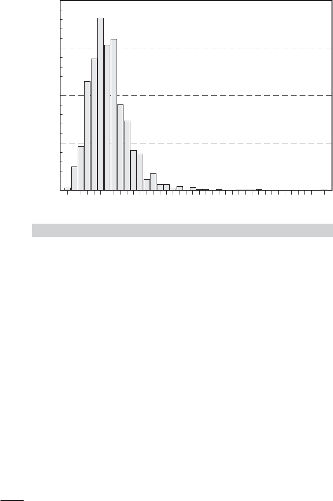
Income

Histogram for Household Income in 1988 GSOEP

0.005 0.290 0.575 0.860 1.145 1.430 1.715 2.000

800

600

400

Frequency

200

FIGURE 7.1

Histogram for Income.

This shows that an alternative way to handle the Box–Cox regression model is to transform

the model into a nonlinear regression and then use the Gauss–Newton regression (see Sec-

tion 7.2.6) to estimate the parameters. The original parameters of the model can be recovered

by λ = γ, α = α

∗

+ 1/γ and β = γβ

∗

Example 7.6 Interaction Effects in a Loglinear Model for Income

A recent study in health economics is “Incentive Effects in the Demand for Health Care:

A Bivariate Panel Count Data Estimation” by Riphahn, Wambach, and Million (2003). The

authors were interested in counts of physician visits and hospital visits and in the impact that

the presence of private insurance had on the utilization counts of interest, that is, whether

the data contain evidence of moral hazard. The sample used is an unbalanced panel of 7,293

households, the German Socioeconomic Panel (GSOEP) data set.

Among the variables re-

ported in the panel are household income, with numerous other sociodemographic variables

such as age, gender, and education. For this example, we will model the distribution of in-

come using the last wave of the data set (1988), a cross section with 4,483 observations.

Two of the individuals in this sample reported zero income, which is incompatible with the

underlying models suggested in the development below. Deleting these two observations

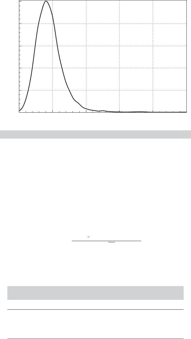
leaves a sample of 4,481 observations. Figures 7.1 and 7.2 display a histogram and a kernel

density estimator for the household income variable for these observations.

We will ﬁt an exponential regression model to the income variable, with

Income = exp( β

+ β

Age + β

Age

+ β

Education + β

Female

+ β

Female × Education + β

Age × Education) + ε.

The data are published on the Journal of Applied Econometrics data archive Web site, at

http://qed.econ.queensu.ca/jae/2003-v18.4/riphahn-wambach-million/. The variables in the data ﬁle are listed

in Appendix Table F7.1. The number of observations in each year varies from one to seven with a total

number of 27,326 observations. We will use these data in several examples here and later in the book.

196

PART I

✦

The Linear Regression Model

Income

0.57

1.14

1.71

2.28

2.85

0.00

0.41 0.82 1.23 1.64 2.050.00

Density

FIGURE 7.2

Kernel Density Estimate for Income.

Table 7.2 provides descriptive statistics for the variables used in this application.

Loglinear models play a prominent role in statistics. Many derive from a density function

of the form f ( y|x) = p[y|α

+ x



β, θ ], where α

is a constant term and θ is an additional

parameter, and

E[y|x] = g( θ) exp(α

+ x



β),

(hence the name “loglinear models”). Examples include the Weibull, gamma, lognormal, and

exponential models for continuous variables and the Poisson and negative binomial models

for counts. We can write E[y|x] as exp[ln g(θ ) + α

+ x



β], and then absorb lng(θ) in the

constant term in ln E[y |x] = α + x



β. The lognormal distribution (see Section B.4.4) is often

used to model incomes. For the lognormal random variable,

p[y|α

+ x



β, θ ] =

exp[−

(lny − α

− x



β)

/θ

]

θ y

√

2π

, y > 0,

E[y|x] = exp(α

+ x



β + θ

/2) = exp( α + x



β).

TABLE 7.2

Descriptive Statistics for Variables Used in

Nonlinear Regression

Variable Mean Std.Dev. Minimum Maximum

INCOME 0.348896 0.164054 0.0050 2

AGE 43.4452 11.2879 25 64

EDUC 11.4167 2.36615 7 18

FEMALE 0.484267 0.499808 0 1

CHAPTER 7

✦

Nonlinear, Semiparametric, Nonparametric Regression

197

The exponential regression model is also consistent with a gamma distribution. The density

of a gamma distributed random variable is

p[y|α

+ x



β, θ ] =

exp(−λy) y

θ−1

( θ)

, y > 0, θ>0, λ = exp( −α

− x



β),

E[y|x] = θ/λ = θ exp(α

+ x



β) = exp(ln θ + α

+ x



β) = exp(α + x



β).

The parameter θ determines the shape of the distribution. When θ>2, the gamma density

has the shape of a chi-squared variable (which is a special case). Finally, the Weibull model

has a similar form,

p[y|α

+ x



β, θ ] = θλ

exp[−(λy)

θ−1

, y ≥ 0, θ>0, λ = exp( −α

− x



β),

E[y|x] = (1 + 1/θ) exp(α

+ x



β) = exp[ln (1+ 1/θ) + α

+ x



β] = exp(α + x



β).

In all cases, the maximum likelihood estimator is the most efﬁcient estimator of the pa-

rameters. (Maximum likelihood estimation of the parameters of this model is considered in

Chapter 14.) However, nonlinear least squares estimation of the model

E[y|x] = exp(α + x



β) + ε

has a virtue in that the nonlinear least squares estimator will be consistent even if the dis-

tributional assumption is incorrect—it is robust to this type of misspeciﬁcation since it does

not make explicit use of a distributional assumption.

Table 7.3 presents the nonlinear least squares regression results. Superﬁcially, the pattern

of signs and signiﬁcance might be expected—with the exception of the dummy variable for

female. However, two issues complicate the interpretation of the coefﬁcients in this model.

First, the model is nonlinear, so the coefﬁcients do not give the magnitudes of the interesting

effects in the equation. In particular, for this model,

∂ E[y|x]/∂ x

= exp(α + x



β) × ∂(α + x



β)/∂ x

Second, as we have constructed our model, the second part of the derivative is not equal to

the coefﬁcient, because the variables appear either in a quadratic term or as a product with

some other variable. Moreover, for the dummy variable, Female, we would want to compute

the partial effect using

E[y|x]/Female = E[y|x, Female = 1] − E[y|x, Female = 0]

A third consideration is how to compute the partial effects, as sample averages or at the

means of the variables. For example,

∂ E[y|x]/∂Age = E[y|x] × ( β

+ 2β

Age + β

Educ).

TABLE 7.3

Estimated Regression Equations

Nonlinear Least Squares Linear Least Squares

Variable Estimate Std. Error t Estimate Std. Error t

Constant −2.58070 0.17455 14.78 −0.13050 0.06261 −2.08

Age 0.06020 0.00615 9.79 0.01791 0.00214 8.37

Age

−0.00084 0.00006082 −13.83 −0.00027 0.00001985 −13.51

Education −0.00616 0.01095 −0.56 −0.00281 0.00418 −0.67

Female 0.17497 0.05986 2.92 0.07955 0.02339 3.40

Female × Educ −0.01476 0.00493 −2.99 −0.00685 0.00202 −3.39

Age × Educ 0.00134 0.00024 5.59 0.00055 0.00009394 5.88



e 106.09825 106.24323

s 0.15387 0.15410

0.12005 0.11880

198

PART I

✦

The Linear Regression Model

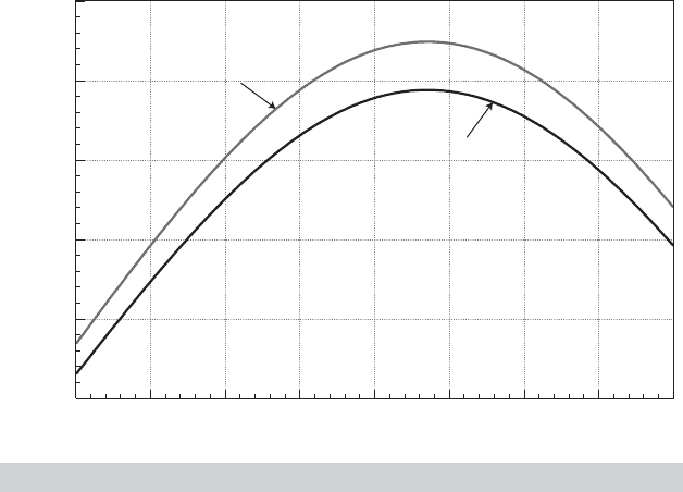
Years

Expected Income vs. Age for Men and Women with Educ = 16

0.328

0.376

0.425

0.474

0.522

0.279

30 35 40 45 50 55 60 6525

Expected Income

Women

Men

FIGURE 7.3

Expected Incomes.

The average value of Age in the sample is 43.4452 and the average Education is 11.4167.

The partial effect of a year of education is estimated to be 0.000948 if it is computed by

computing the partial effect for each individual and averaging the result. It is 0.000925 if it

is computed by computing the conditional mean and the linear term at the averages of the

three variables. The partial effect is difﬁcult to interpret without information about the scale of

the income variable. Since the average income in the data is about 0.35, these partial effects

suggest that an additional year of education is associated with a change in expected income

of about 2.6 percent (i.e., 0.009/0.35).

The rough calculation of partial effects with respect to Age does not reveal the model

implications about the relationship between age and expected income. Note, for example,

that the coefﬁcient on Age is positive while the coefﬁcient on Age

is negative. This implies

(neglecting the interaction term at the end), that the Age − Income relationship implied by the

model is parabolic. The partial effect is positive at some low values and negative at higher

values. To explore this, we have computed the expected Income using the model separately

for men and women, both with assumed college education (Educ = 16) and for the range of

ages in the sample, 25 to 64. Figure 7.3 shows the result of this calculation. The upper curve

is for men (Female = 0) and the lower one is for women. The parabolic shape is as expected;

what the ﬁgure reveals is the relatively strong effect—ceteris paribus, incomes are predicted

to rise by about 80 percent between ages 25 and 48. (There is an important aspect of this

computation that the model builder would want to develop in the analysis. It remains to be

argued whether this parabolic relationship describes the trajectory of expected income for

an individual as they age, or the average incomes of different cohorts at a particular moment

in time (1988). The latter would seem to be the more appropriate conclusion at this point,

though one might be tempted to infer the former.)

The ﬁgure reveals a second implication of the estimated model that would not be obvious

from the regression results. The coefﬁcient on the dummy variable for Female is positive,

highly signiﬁcant, and, in isolation, by far the largest effect in the model. This might lead

the analyst to conclude that on average, expected incomes in these data are higher for

women than men. But, Figure 7.3 shows precisely the opposite. The difference is accounted