Greene W.H. Econometric Analysis

Подождите немного. Документ загружается.

FUNCTIONAL FORM AND

STRUCTURAL CHANGE

6.1 INTRODUCTION

This chapter will complete our analysis of the linear regression model. We begin by ex-

amining different aspects of the functional form of the regression model. Many different

types of functions are linear by the deﬁnition in Section 2.3.1. By using different trans-

formations of the dependent and independent variables, binary variables, and different

arrangements of functions of variables, a wide variety of models can be constructed that

are all estimable by linear least squares. Section 6.2 considers using binary variables to

accommodate nonlinearities in the model. Section 6.3 broadens the class of models

that are linear in the parameters. By using logarithms, quadratic terms, and interaction

terms (products of variables), the regression model can accommodate a wide variety of

functional forms in the data.

Section 6.4 examines the issue of specifying and testing for discrete change in the

underlying process that generates the data, under the heading of structural change.In

a time-series context, this relates to abrupt changes in the economic environment, such

as major events in ﬁnancial (e.g., the world ﬁnancial crisis of 2007–2009) or commodity

markets (such as the several upheavals in the oil market). In a cross section, we can

modify the regression model to account for discrete differences across groups such as

different preference structures or market experiences of men and women.

6.2 USING BINARY VARIABLES

One of the most useful devices in regression analysis is the binary,ordummy variable.

A dummy variable takes the value one for some observations to indicate the presence

of an effect or membership in a group and zero for the remaining observations. Bi-

nary variables are a convenient means of building discrete shifts of the function into a

regression model.

6.2.1 BINARY VARIABLES IN REGRESSION

Dummy variables are usually used in regression equations that also contain other quan-

titative variables. In the earnings equation in Example 5.2, we included a variable Kids

to indicate whether there were children in the household, under the assumption that for

many married women, this fact is a signiﬁcant consideration in labor supply behavior.

The results shown in Example 6.1 appear to be consistent with this hypothesis.

149

150

PART I

✦

The Linear Regression Model

TABLE 6.1

Estimated Earnings Equation

ln earnings = β

+ β

age +β

age

+ β

education +β

kids +ε

Sum of squared residuals: 599.4582

Standard error of the regression: 1.19044

based on 428 observations 0.040995

Variable Coefﬁcient Standard Error t Ratio

Constant 3.24009 1.7674 1.833

Age 0.20056 0.08386 2.392

Age

−0.0023147 0.00098688 −2.345

Education 0.067472 0.025248 2.672

Kids −0.35119 0.14753 −2.380

Example 6.1 Dummy Variable in an Earnings Equation

Table 6.1 following reproduces the estimated earnings equation in Example 5.2. The variable

Kids is a dummy variable, which equals one if there are children under 18 in the household and

zero otherwise. Since this is a semilog equation, the value of −0.35 for the coefﬁcient is an

extremely large effect, one which suggests that all other things equal, the earnings of women

with children are nearly a third less than those without. This is a large difference, but one that

would certainly merit closer scrutiny. Whether this effect results from different labor market

effects that inﬂuence wages and not hours, or the reverse, remains to be seen. Second, having

chosen a nonrandomly selected sample of those with only positive earnings to begin with,

it is unclear whether the sampling mechanism has, itself, induced a bias in this coefﬁcient.

Dummy variables are particularly useful in loglinear regressions. In a model of the

form

ln y = β

+ β

x + β

d + ε,

the coefﬁcient on the dummy variable, d, indicates a multiplicative shift of the function.

The percentage change in E[y|x,d] asociated with the change in d is



E[y|x, d]/d



= 100%



E[y|x, d = 1] − E[y|x, d = 0]

E[y|x, d = 0]



= 100%



exp(β

+ β

x + β

)E[exp(ε)] − exp(β

+ β

x)E[exp(ε)]

exp(β

+ β

x)E[exp(ε)]



= 100%

[

exp(β

) − 1

]

Example 6.2 Value of a Signature

In Example 4.10 we explored the relationship between (log of) sale price and surface area for

430 sales of Monet paintings. Regression results from the example are included in Table 6.2.

The results suggest a strong relationship between area and price—the coefﬁcient is 1.33372

indicating a highly elastic relationship and the t ratio of 14.70 suggests the relationship is

highly signiﬁcant. A variable (effect) that is clearly left out of the model is the effect of the

artist’s signature on the sale price. Of the 430 sales in the sample, 77 are for unsigned

paintings. The results at the right of Table 6.2 include a dummy variable for whether the

painting is signed or not. The results show an extremely strong effect. The regression results

imply that

E[Price|Area, Aspect, Signature) =

exp[−9.64 + 1.35 ln Area − 0.08AspectRatio + 1.23Signature + 0.993

/2].

CHAPTER 6

✦

Functional Form and Structural Change

151

TABLE 6.2

Estimated Equations for Log Price

ln price = β

+ β

ln Area +β

aspect ratio +β

signature +ε

Mean of ln Price 0.33274

Number of observations 430

Sum of squared residuals 519.17235 420.16787

Standard error 1.10266 0.99313

R-squared 0.33620 0.46279

Adjusted R-squared 0.33309 0.45900

Standard Standard

Variable Coefﬁcient Error t Coefﬁcient Error t

Constant −8.42653 0.61183 −13.77 −9.64028 0.56422 −17.09

Ln area 1.33372 0.09072 14.70 1.34935 0.08172 16.51

Aspect ratio −0.16537 0.12753 −1.30 −0.07857 0.11519 −0.68

Signature 0.00000 0.00000 0.00 1.25541 0.12530 10.02

(See Section 4.6.) Computing this result for a painting of the same area and aspect ratio, we

ﬁnd the model predicts that the signature effect would be

100% × ( E[Price]/Price) = 100%[exp( 1.26) − 1] = 252%.

The effect of a signature on an otherwise similar painting is to more than double the price. The

estimated standard error for the signature coefﬁcient is 0.1253. Using the delta method, we

obtain an estimated standard error for [exp( b

) −1] of the square root of [exp(b

)]

×.1253

which is 0.4417. For the percentage difference of 252%, we have an estimated standard

error of 44.17%.

Superﬁcially, it is possible that the size effect we observed earlier could be explained by

the presence of the signature. If the artist tended on average to sign only the larger paintings,

then we would have an explanation for the counterintuitive effect of size. (This would be

an example of the effect of multicollinearity of a sort.) For a regression with a continuous

variable and a dummy variable, we can easily conﬁrm or refute this proposition. The average

size for the 77 sales of unsigned paintings is 1,228.69 square inches. The average size of

the other 353 is 940.812 square inches. There does seem to be a substantial systematic

difference between signed and unsigned paintings, but it goes in the other direction. We

are left with signiﬁcant ﬁndings of both a size and a signature effect in the auction prices of

Monet paintings. Aspect Ratio, however, appears still to be inconsequential.

There is one remaining feature of this sample for us to explore. These 430 sales involved

only 387 different paintings. Several sales involved repeat sales of the same painting. The

assumption that observations are independent draws is violated, at least for some of them.

We will examine this form of “clustering” in Chapter 11 in our treatment of panel data.

It is common for researchers to include a dummy variable in a regression to account

for something that applies only to a single observation. For example, in time-series

analyses, an occasional study includes a dummy variable that is one only in a single

unusual year, such as the year of a major strike or a major policy event. (See, for

example, the application to the German money demand function in Section 21.3.5.) It

is easy to show (we consider this in the exercises) the very useful implication of this:

A dummy variable that takes the value one only for one observation has the effect of

deleting that observation from computation of the least squares slopes and variance

estimator (but not R-squared).

152

PART I

✦

The Linear Regression Model

6.2.2 SEVERAL CATEGORIES

When there are several categories, a set of binary variables is necessary. Correcting

for seasonal factors in macroeconomic data is a common application. We could write a

consumption function for quarterly data as

= β

+ β

+ δ

+ ε

where x

is disposable income. Note that only three of the four quarterly dummy vari-

ables are included in the model. If the fourth were included, then the four dummy

variables would sum to one at every observation, which would reproduce the constant

term—a case of perfect multicollinearity. This is known as the dummy variable trap.

Thus, to avoid the dummy variable trap, we drop the dummy variable for the fourth quar-

ter. (Depending on the application, it might be preferable to have four separate dummy

variables and drop the overall constant.)

Any of the four quarters (or 12 months) can

be used as the base period.

The preceding is a means of deseasonalizing the data. Consider the alternative

formulation:

= βx

+ δ

+ ε

. (6-1)

Using the results from Section 3.3 on partitioned regression, we know that the preceding

multiple regression is equivalent to ﬁrst regressing C and x on the four dummy variables

and then using the residuals from these regressions in the subsequent regression of

deseasonalized consumption on deseasonalized income. Clearly, deseasonalizing in this

fashion prior to computing the simple regression of consumption on income produces

the same coefﬁcient on income (and the same vector of residuals) as including the set

of dummy variables in the regression.

Example 6.3 Genre Effects on Movie Box Ofﬁce Receipts

Table 4.8 in Example 4.12 presents the results of the regression of log of box ofﬁce receipts

for 62 2009 movies on a number of variables including a set of dummy variables for genre:

Action, Comedy, Animated,orHorror. The left out category is “any of the remaining 9 genres”

in the standard set of 13 that is usually used in models such as this one. The four coefﬁcients

are −0.869, −0.016, −0.833, +0.375, respectively. This suggests that, save for horror movies,

these genres typically fare substantially worse at the box ofﬁce than other types of movies.

We note the use of b directly to estimate the percentage change for the category, as we

did in example 6.1 when we interpreted the coefﬁcient of −0.35 on Kids as indicative of a

35 percent change in income, is an approximation that works well when b is close to zero

but deteriorates as it gets far from zero. Thus, the value of −0.869 above does not translate

to an 87 percent difference between Action movies and other movies. Using the formula we

used in Example 6.2, we ﬁnd an estimated difference closer to [exp( −0.869) − 1] or about

58 percent.

6.2.3 SEVERAL GROUPINGS

The case in which several sets of dummy variables are needed is much the same as

those we have already considered, with one important exception. Consider a model of

statewide per capita expenditure on education y as a function of statewide per capita

income x. Suppose that we have observations on all n = 50 states for T = 10 years.

See Suits (1984) and Greene and Seaks (1991).

CHAPTER 6

✦

Functional Form and Structural Change

153

A regression model that allows the expected expenditure to change over time as well

as across states would be

= α + β x

+ δ

+ θ

+ ε

. (6-2)

As before, it is necessary to drop one of the variables in each set of dummy variables

to avoid the dummy variable trap. For our example, if a total of 50 state dummies and

10 time dummies is retained, a problem of “perfect multicollinearity” remains; the sums

of the 50 state dummies and the 10 time dummies are the same, that is, 1. One of the

variables in each of the sets (or the overall constant term and one of the variables in

one of the sets) must be omitted.

Example 6.4 Analysis of Covariance

The data in Appendix Table F6.1 were used in a study of efﬁciency in production of airline

services in Greene (2007a). The airline industry has been a favorite subject of study [e.g.,

Schmidt and Sickles (1984); Sickles, Good, and Johnson (1986)], partly because of interest

in this rapidly changing market in a period of deregulation and partly because of an abun-

dance of large, high-quality data sets collected by the (no longer existent) Civil Aeronautics

Board. The original data set consisted of 25 ﬁrms observed yearly for 15 years (1970 to 1984),

a “balanced panel.” Several of the ﬁrms merged during this period and several others expe-

rienced strikes, which reduced the number of complete observations substantially. Omitting

these and others because of missing data on some of the variables left a group of 10 full

observations, from which we have selected six for the examples to follow. We will ﬁt a cost

equation of the form

ln C

i,t

= β

+ β

ln Q

i,t

+ β

i,t

+ β

ln P

fuel i,t

+ β

Loadfactor

i,t



t=1

i,t



i =1

i,t

+ ε

i,t

The dummy variables are D

i,t

which is the year variable and F

i,t

which is the ﬁrm variable. We

have dropped the last one in each group. The estimated model for the full speciﬁcation is

ln C

i,t

= 13.56 + 0.8866 ln Q

i,t

+ 0.01261 ln

i,t

+ 0.1281 ln P

fi,t

− 0.8855 LF

i,t

+time effects + ﬁrm effects + e

i,t

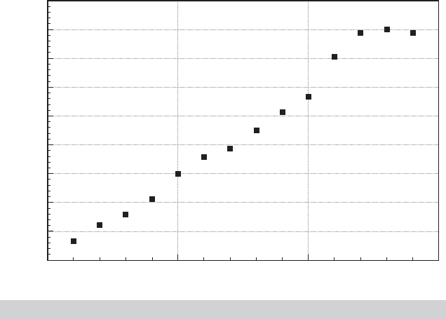
The year effects display a revealing pattern, as shown in Figure 6.1. This was a period of

rapidly rising fuel prices, so the cost effects are to be expected. Since one year dummy

variable is dropped, the effect shown is relative to this base year (1984).

We are interested in whether the ﬁrm effects, the time effects, both, or neither are sta-

tistically signiﬁcant. Table 6.3 presents the sums of squares from the four regressions. The

F statistic for the hypothesis that there are no ﬁrm-speciﬁc effects is 65.94, which is highly

signiﬁcant. The statistic for the time effects is only 2.61, which is larger than the critical value

of 1.84, but perhaps less so than Figure 6.1 might have suggested. In the absence of the

TABLE 6.3

tests for Firm and Year Effects

Model Sum of Squares Restrictions F Deg.Fr.

Full model 0.17257 0 —

Time effects only 1.03470 5 65.94 [5, 66]

Firm effects only 0.26815 14 2.61 [14, 66]

No effects 1.27492 19 22.19 [19, 66]

154

PART I

✦

The Linear Regression Model

0.1

0.0

0.1

0.2

0.3

0.4

0.5

0.6

0.7

0.8

Year

B (Year)

10 15

FIGURE 6.1

Estimated Year Dummy Variable Coefﬁcients.

year-speciﬁc dummy variables, the year-speciﬁc effects are probably largely absorbed by

the price of fuel.

6.2.4 THRESHOLD EFFECTS AND CATEGORICAL VARIABLES

In most applications, we use dummy variables to account for purely qualitative factors,

such as membership in a group, or to represent a particular time period. There are cases,

however, in which the dummy variable(s) represents levels of some underlying factor

that might have been measured directly if this were possible. For example, education

is a case in which we typically observe certain thresholds rather than, say, years of

education. Suppose, for example, that our interest is in a regression of the form

income = β

+ β

age + effect of education + ε.

The data on education might consist of the highest level of education attained, such

as high school (HS), undergraduate (B), master’s (M), or Ph.D. (P). An obviously

unsatisfactory way to proceed is to use a variable E that is 0 for the ﬁrst group, 1 for the

second, 2 for the third, and 3 for the fourth. That is, income = β

+ β

age + β

E + ε.

The difﬁculty with this approach is that it assumes that the increment in income at each

threshold is the same; β

is the difference between income with a Ph.D. and a master’s

and between a master’s and a bachelor’s degree. This is unlikely and unduly restricts

the regression. A more ﬂexible model would use three (or four) binary variables, one

for each level of education. Thus, we would write

income = β

+ β

age + δ

B + δ

M + δ

P + ε.

CHAPTER 6

✦

Functional Form and Structural Change

155

The correspondence between the coefﬁcients and income for a given age is

High school: E [income |age, HS] = β

+ β

age,

Bachelor’s: E [income |age, B] = β

+ β

age + δ

Master’s: E [income |age, M] = β

+ β

age + δ

Ph.D.: E [income |age, P] = β

+ β

age + δ

The differences between, say, δ

and δ

and between δ

and δ

are of interest. Obvi-

ously, these are simple to compute. An alternative way to formulate the equation that

reveals these differences directly is to redeﬁne the dummy variables to be 1 if the indi-

vidual has the degree, rather than whether the degree is the highest degree obtained.

Thus, for someone with a Ph.D., all three binary variables are 1, and so on. By deﬁning

the variables in this fashion, the regression is now

High school: E [income |age, HS] = β

+ β

age,

Bachelor’s: E [income |age, B] = β

+ β

age + δ

Master’s: E [income |age, M] = β

+ β

age + δ

+ δ

Ph.D.: E [income |age, P] = β

+ β

age + δ

+ δ

Instead of the difference between a Ph.D. and the base case, in this model δ

is the

marginal value of the Ph.D. How equations with dummy variables are formulated is a

matter of convenience. All the results can be obtained from a basic equation.

6.2.5 TREATMENT EFFECTS AND DIFFERENCE

IN DIFFERENCES REGRESSION

Researchers in many ﬁelds have studied the effect of a treatment on some kind of

response. Examples include the effect of going to college on lifetime income [Dale

and Krueger (2002)], the effect of cash transfers on child health [Gertler (2004)], the

effect of participation in job training programs on income [LaLonde (1986)], and pre-

versus postregime shifts in macroeconomic models [Mankiw (2006)], to name but a

few. These examples can be formulated in regression models involving a single dummy

variable:

= x



β + δ D

+ ε

where the shift parameter, δ, measures the impact of the treatment or the policy change

(conditioned on x) on the sampled individuals. In the simplest case of a comparison of

one group to another,

= β

+ β

+ ε

we will have b

= ( ¯y|D

= 0), that is, the average outcome of those who did not ex-

perience the intervention, and b

= ( ¯y|D

= 1) − ( ¯y|D

= 0), the difference in the

means of the two groups. In the Dale and Krueger (2002) study, the model compared

the incomes of students who attended elite colleges to those who did not. When the

analysis is of an intervention that occurs over time, such as Krueger’s (1999) analysis

of the Tennessee STAR experiment in which school performance measures were ob-

served before and after a policy dictated a change in class sizes, the treatment dummy

156

PART I

✦

The Linear Regression Model

variable will be a period indicator, D

= 0 in period 1 and 1 in period 2. The effect in β

measures the change in the outcome variable, for example, school performance, pre- to

postintervention; b

= ¯y

− ¯y

The assumption that the treatment group does not change from period 1 to period 2

weakens this comparison. A strategy for strengthening the result is to include in the

sample a group of control observations that do not receive the treatment. The change in

the outcome for the treatment group can then be compared to the change for the control

group under the presumption that the difference is due to the intervention. An intriguing

application of this strategy is often used in clinical trials for health interventions to

accommodate the placebo effect. The placebo “effect” is a controversial, but apparently

tangible outcome in some clinical trials in which subjects “respond” to the treatment

even when the treatment is a decoy intervention, such as a sugar or starch pill in a drug

trial. [See Hr ´objartsson and G ¨otzsche, 2001.] A broad template for assessment of the

results of such a clinical trial is as follows: The subjects who receive the placebo are

the controls. The outcome variable—level of cholesterol for example—is measured at

the baseline for both groups. The treatment group receives the drug; the control group

receives the placebo, and the outcome variable is measured posttreatment. The impact

is measured by the difference in differences,

E = [( ¯y

exit

|treatment) − ( ¯y

baseline

|treatment)] − [( ¯y

exit

|placebo) − ( ¯y

baseline

|placebo)].

The presumption is that the difference in differences measurement is robust to the

placebo effect if itexists. If there is no placebo effect, the result is even stronger

(assuming there is a result).

An increasingly common social science application of treatment effect models with

dummy variables is in the evaluation of the effects of discrete changes in policy.

pioneering application is the study of the Manpower Development and Training Act

(MDTA) by Ashenfelter and Card (1985). The simplest form of the model is one with

a pre- and posttreatment observation on a group, where the outcome variable is y,

with

= β

+ β

× D

+ ε

, t = 1, 2. (6-3)

In this model, T

is a dummy variable that is zero in the pretreatment period and

one after the treatment and D

equals one for those individuals who received the

“treatment.” The change in the outcome variable for the “treated” individuals will

= 1) − (y

= 1) = (β

+ β

) − (β

+ β

) = β

+ β

For the controls, this is

= 0) − (y

= 0) = (β

+ β

) − (β

) = β

The difference in differences is

[(y

= 1) − (y

= 1)] − [(y

= 0) − (y

= 0)] = β

Surveys of literatures on treatment effects, including use of, ‘D-i-D,’ estimators, are provided by Imbens and

Wooldridge (2009) and Millimet, Smith, and Vytlacil (2008).

CHAPTER 6

✦

Functional Form and Structural Change

157

In the multiple regression of y

on a constant, T, D, and TD, the least squares estimate

of β

will equal the difference in the changes in the means,

(

¯y|D = 1, Period 2

)

−

(

¯y|D = 1, Period 1

)

−

(

¯y|D = 0, Period 2

)

−

(

¯y|D = 0, Period 1

)

=  ¯y|treatment −  ¯y|control.

The regression is called a difference in differences estimator in reference to this result.

When the treatment is the result of a policy change or event that occurs completely

outside the context of the study, the analysis is often termed a natural experiment. Card’s

(1990) study of a major immigration into Miami in 1979 discussed in Example 6.5 is an

application.

Example 6.5 A Natural Experiment: The Mariel Boatlift

A sharp change in policy can constitute a natural experiment. An example studied by Card

(1990) is the Mariel boatlift from Cuba to Miami (May–September 1980), which increased the

Miami labor force by 7 percent. The author examined the impact of this abrupt change in labor

market conditions on wages and employment for nonimmigrants. The model compared Miami

to a similar city, Los Angeles. Let i denote an individual and D denote the “treatment,” which

for an individual would be equivalent to “lived in a city that experienced the immigration.”

For an individual in either Miami or Los Angeles, the outcome variable is

) = 1 if they are unemployed and 0 if they are employed.

Let c denote the city and let t denote the period, before (1979) or after (1981) the immigration.

Then, the unemployment rate in city c at time t is E[y

i,0

|c, t] if there is no immigration and it

is E[y

i,1

|c, t] if there is the immigration. These rates are assumed to be constants. Then,

E[ y

i,0

|c, t] = β

+ γ

without the immigration,

E[ y

i,1

|c, t] = β

+ γ

+ δ with the immigration.

The effect of the immigration on the unemployment rate is measured by δ. The natural ex-

periment is that the immigration occurs in Miami and not in Los Angeles but is not a result

of any action by the people in either city. Then,

E[ y

|M, 79] = β

+ γ

and E[ y

|M, 81] = β

+ γ

+ δ for Miami,

E[ y

|L, 79] = β

+ γ

and E[ y

|L, 81] = β

+ γ

for Los Angeles.

It is assumed that unemployment growth in the two cities would be the same if there were

no immigration. If neither city experienced the immigration, the change in the unemployment

rate would be

E[ y

i,0

|M, 81] − E[ y

i,0

|M, 79] = β

− β

for Miami,

E[ y

i,0

|L, 81] − E[ y

i,0

|L, 79] = β

− β

for Los Angeles.

If both cities were exposed to migration,

E[ y

i,1

|M, 81] − E[ y

i,1

|M, 79] = β

− β

+ δ for Miami

E[ y

i,1

|L, 81] − E[ y

i,1

|L, 79] = β

− β

+ δ for Los Angeles.

Only Miami experienced the migration (the “treatment”). The difference in differences that

quantiﬁes the result of the experiment is

{E[ y

i,1

|M, 81] − E[ y

i,1

|M, 79]}−{E[ y

i,0

|L, 81] − E[ y

i,0

|L, 79]}=δ.

158

PART I

✦

The Linear Regression Model

The author examined changes in employment rates and wages in the two cities over several

years after the boatlift. The effects were surprisingly modest given the scale of the experiment

in Miami.

One of the important issues in policy analysis concerns measurement of such treat-

ment effects when the dummy variable results from an individual participation decision.

In the clinical trial example given earlier, the control observations (it is assumed) do not

know they they are in the control group. The treatment assignment is exogenous to the

experiment. In contrast, in Keueger and Dale’s study, the assignment to the treatment

group, attended the elite college, is completely voluntary and determined by the indi-

vidual. A crucial aspect of the analysis in this case is to accommodate the almost certain

outcome that the “treatment dummy” might be measuring the latent motivation and

initiative of the participants rather than the effect of the program itself. That is the main

appeal of the natural experiment approach—it more closely (possibly exactly) repli-

cates the exogenous treatment assignment of a clinical trial.

We will examine some of

these cases in Chapters 8 and 19.

6.3 NONLINEARITY IN THE VARIABLES

It is useful at this point to write the linear regression model in a very general form: Let

z = z

, z

,...,z

be a set of L independent variables; let f

, f

,..., f

be K linearly

independent functions of z; let g(y) be an observable function of y; and retain the usual

assumptions about the disturbance. The linear regression model may be written

g(y) = β

(z) + β

(z) +···+β

(z) + ε

= β

+ β

+···+β

+ ε

= x



β + ε.

(6-4)

By using logarithms, exponentials, reciprocals, transcendental functions, polynomials,

products, ratios, and so on, this “linear” model can be tailored to any number of

situations.

6.3.1 PIECEWISE LINEAR REGRESSION

If one is examining income data for a large cross section of individuals of varying ages

in a population, then certain patterns with regard to some age thresholds will be clearly

evident. In particular, throughout the range of values of age, income will be rising,but the

slope might change at some distinct milestones, for example, at age 18, when the typical

individual graduates from high school, and at age 22, when he or she graduates from

college. The time proﬁle of income for the typical individual in this population might

appear as in Figure 6.2. Based on the discussion in the preceding paragraph, we could

ﬁt such a regression model just by dividing the sample into three subsamples. However,

this would neglect the continuity of the proposed function. The result would appear

more like the dotted ﬁgure than the continuous function we had in mind. Restricted

See Angrist and Krueger (2001) and Angrist and Pischke (2010) for discussions of this approach.