Geiser J. Decomposition Methods for Differential Equations: Theory and Applications

Подождите немного. Документ загружается.

Time-Decomposition Methods for Parabolic Equations for Parabolic Equations 45

Cauchy problem:

∂

c(t)=Ac(t)+Bc(t), 0 <t≤ T,

c(0) = c

(3.30)

Then the problem (3.30) has a unique solution. The iteration (3.28)–(3.29) for

i =1, 3,...,2m +1is consistent with the order of the consistency O(τ

2m+1

PROOF

Because A + B ∈L(X), it is a generator of a uniformly continuous

semigroup; hence, the problem (3.30) has a unique solution c(t)=exp((A +

B)t)c

Let us consider the iteration (3.28)–(3.29) on the subinterval [t

n+1

]. For

the local error function e

(t)=c(t) − c

(t), we have the following relations:

∂

(t)=Ae

(t)+Be

i−1

(t),t∈ (t

n+1

)=0,

(3.31)

and

∂

i+1

(t)=Ae

(t)+Be

i+1

(t),t∈ (t

n+1

i+1

)=0,

(3.32)

for i =1, 3, 5,...,withe

(0) = 0 and e

(t)=c(t). We use the notation X

for

the product space X × X supplied with the norm (u, v) =max{u, v}

(u, v ∈ X). The elements E

(t), F

(t) ∈ X

and the linear operator A : X

→

are deﬁned as follows:

(t)=



(t)

i+1

(t)



, F

(t)=



i−1

(t)



, A =



A 0



. (3.33)

Then, using the notations (3.33), the relations (3.31)–(3.32) can be written in

the form

∂

(t)=AE

(t)+F

(t),t∈ (t

n+1

)=0.

(3.34)

Because of our assumptions, A is a generator of the one-parameter C

semi-

group (exp At)

t≥0

. Hence, by using the variations of constants formula, the

solution of the abstract Cauchy problem (3.34) with homogeneous initial con-

ditions can be written as

(t)=



exp(A(t − s))F

(s)ds, t ∈ [t

n+1

(3.35)

Then, using the denotation

E



∞

=sup

t∈[t

n+1

]

E

(t),

(3.36)

46Decomposition Methods for Diﬀerential Equations Theory and Applications

we have

E

(t)≤F



∞



exp(A(t − s))ds

= Be

i−1





exp(A(t − s))ds, t ∈ [t

n+1

(3.37)

Because (A(t))

t≥0

is a semigroup, the growth estimation,

exp(At)≤K exp(ωt); t ≥ 0,

(3.38)

holds with some numbers K ≥ 0andω ∈ R.

• Assume that (A(t))

t≥0

is a bounded or exponentially stable semigroup;

that is, (3.38) holds for some ω ≤ 0. Then obviously the estimate

exp(At)≤K, t ≥ 0,

(3.39)

holds, and hence, according to (3.37), we have the relation

E

(t) ≤ KBτ

e

i−1

,t∈ [t

n+1

(3.40)

• Assume that (exp At)

t≥0

has an exponential growth with some ω>0.

Using (3.38) we have



exp(A(t − s))ds ≤ K

(t),t∈ [t

n+1

(3.41)

where

(t)=

(exp(ω(t − t

)) − 1) ,t∈ [t

n+1

(3.42)

Hence,

(t) ≤

(exp(ωτ

) − 1) = Kτ

+ O(τ

(3.43)

The estimations (3.40) and (3.43) result in

E



∞

= K Bτ

e

i−1

 + O(τ

(3.44)

Taking into account the deﬁnition of E

and the norm ·

∞

(supremum norm),

we obtain

e

 = KBτ

e

i−1

 + O(τ

(3.45)

and consequently,

e

i+1

 = K B||e



exp(A(t − s))ds, (3.46)

= KBτ

(KBτ

e

i−1

 + O(τ

)),

= K

e

i−1

 + O(τ

Time-Decomposition Methods for Parabolic Equations for Parabolic Equations 47

We apply the recursive argument that proves our statement.

REMARK 3.7 When A and B are matrices (i.e., when (3.28)–(3.29)

is a system of the ordinary diﬀerential equations), we can use the concept

of the logarithmic norm for the growth estimation (3.38). Hence, for many

important classes of matrices, we can prove the validity of (3.38) with ω ≤ 0.

REMARK 3.8 We note that a huge class of important diﬀerential

operators generate a contractive semigroup. This means that for such prob-

lems, assuming the exact solvability of the split subproblems, the iterative

splitting method is convergent to the exact solution in second order.

REMARK 3.9 We note that the assumption A ∈L(X)canbefor-

mulated more weakly as it is enough to assume that the operator A is the

generator of a C

semigroup.

REMARK 3.10 When T is a suﬃciently small number, then we do

not need to partition the interval [0,T] into the subintervals. In this case,

the convergence of the iteration (3.28)–(3.29) to the solution of the problem

(3.30) follows immediately from Theorem 3.1, and the rate of the convergence

is equal to the order of the local splitting error.

REMARK 3.11 Estimate (3.47) shows that after the ﬁnal iteration

step (i =2m + 1), we have the estimation

e

2m+1

 = K

e

τ

+ O(τ

2m+1

). (3.47)

This relation shows that the constant in the leading term strongly depends on

the choice of the initial guess c

(t). When the choice is c

(t) = 0 (see [130]),

then e

 = c(t)(wherec(t) is the exact solution of the original problem) and

hence the error might be signiﬁcant.

REMARK 3.12 In realistic applications, the ﬁnal iteration steps

2m + 1 and the time-step τ

are chosen in an optimal relation to one an-

other, such that the time-step τ

can be chosen maximal and with at least

three or ﬁve iteration steps. Additionally, a ﬁnal stop criterion as an error

bound (e.g., |c

− c

i−1

|≤err with for example err = 10

−4

), helps to restrict

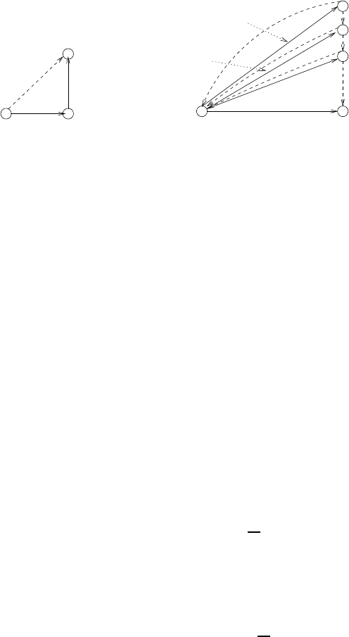
the number of steps. A graphical illustration of the iterative splitting method

is given in Figure 3.4.

48Decomposition Methods for Diﬀerential Equations Theory and Applications

c(t )

Iterative Splitting

with sufficient large iteration

c (t )

n+1

Splitting

Sequential

n+1

c(t ) 1

c (t )

A+B

c (t )~

n+1

A+B

c (t )

n+1

(convergence)

c(t )

FIGURE 3.4: Graphical visualization of noniterative and iterative splitting

methods.

3.2.3.2 Increase of the Order of Accuracy with Improved Initial

Functions

We can increase the order of accuracy by improving our choice of the initial

iteration function, see [69].

Based on our previous assumption about the initial solutions, we start with

exact solutions or an interpolated split solution and present our theory for the

exactness of the method.

The Exact Solution of the Split Subproblem

We derive the exact solution of Equations (3.28) and (3.29) by solving the

ﬁrst split problem,

n+1

)=exp(At)c

∞



s=0

∞



k=s+1

k−s−1

(s)

i−1

), (3.48)

and the second split problem,

i+1

n+1

)=exp(Bt)c

∞



s=0

∞



k=s+1

k−s−1

(s)

), (3.49)

where τ = t

n+1

− t

is the equidistant time-step and c

= c(t

)istheexact

solution at time t

or at least approximately of local order O(τ

m+2

). n is the

number of time-steps (n ∈{0,...,N},N ∈ N

), and m>0isthenumberof

iteration steps.

Time-Decomposition Methods for Parabolic Equations for Parabolic Equations 49

THEOREM 3.2

Assume that for the functions c

i−1

n+1

) and c

n+1

) the conditions

i−1

)=(A + B)

,s=0, 1,...,m+1, (3.50)

)=(A + B)

,s=0, 1,...,m+2, (3.51)

are satisﬁed. After m +2 iterations, the method has a local splitting error

O(τ

m+2

), and therefore the global error err

global

is O(τ

m+1

PROOF

We show that

exp(τ(A + B))c

− c

m+1

n+1

)=O(τ

m+1

), (3.52)

exp(τ(A + B))c

− c

m+2

n+1

)=O(τ

m+2

). (3.53)

Using the assumption and the exact solutions (3.48) and (3.49), we must proof

the relations:

m+1



p=0

(A + B)

m+1



p=0

(A)



s=0

m+1



k=s+1

k−s−1

B, (3.54)

and

m+2



p=0

(A + B)

m+2



p=0

(B)

m+1



s=0

m+2



k=s+1

k−s−1

A. (3.55)

For the proof, we can use the mathematical induction, see [69].

So for each further iteration step, we conserve the order O(τ

m+1

)forEqua-

tion (3.54) or O(τ

m+2

) for Equation (3.55).

We assume for all local errors the order O(τ

m+2

Based on this assumption, we obtain for the global error

err

global

n+1

)=(n +1)err

local

(τ)

=(n +1)τ

err

local

(τ)

= O(τ

m+1

), (3.56)

where we assume equidistant time-steps, a time t

n+1

=(n +1) τ ,andthe

same local error for all n + 1 time-steps, see also [145].

REMARK 3.13 The exact solution of the split subproblem can also

be extended to singular perturbed problems and unbounded operators. In

these cases, a formal solution with respect to the asymptotic convergence of a

power series, which is near the exact solution, can be sought, see [8] and [9].

50Decomposition Methods for Diﬀerential Equations Theory and Applications

Consistency Analysis of the Iterative Operator-Splitting Method

with Interpolated Split Solutions

The algorithm (3.28)–(3.29) requires the knowledge of the functions c

i−1

(t)

and c

(t)onthewholeinterval[t

n+1

]. However, when we solve the split

subproblems, usually we apply some numerical methods that allow us to know

the values of the above functions only at some points of the interval. Hence,

typically we can deﬁne only some interpolations to the exact functions.

In the following we consider and analyze the modiﬁed iterative process

∂c

(t)

∂t

= Ac

(t)+Bc

int

i−1

(t), with c

)=c

, (3.57)

∂c

i+1

(t)

∂t

= Ac

int

(t)+Bc

i+1

(t), with c

i+1

)=c

, (3.58)

where c

int

(t)(fork = i − 1,i) denotes an approximation of the function c

(t)

on the interval [t

n+1

] with the accuracy O(τ

). (For simplicity, we assume

the same order of accuracy with the order p on each subinterval.)

The iteration (3.57)–(3.58) for the error function E

(t) recalls relation (3.33)

with the modiﬁed right side; namely,

(t)=



i−1

(t)+Bh

i−1

(t)



, (3.59)

where h

(t)=c

(t) − c

int

(t)=O(τ

)fork = i − 1,i. Hence,

F



∞

≤ max{Be

i−1

 + h

i−1

; Ah

},

(3.60)

which results in the estimation

F



∞

≤Be

i−1

 + Cτ

(3.61)

Consequently, for these assumptions, the estimation (3.45) turns into the

following:

e

≤K(Bτ

e

i−1

 + Cτ

p+1

)+O(τ

(3.62)

Therefore, for these assumptions the estimation (3.47) takes the modiﬁed

form:

e

i+1

≤K

e

i−1

 + KCτ

p+2

+ KCτ

p+1

+ O(τ

), (3.63)

leading to Theorem 3.3.

THEOREM 3.3

Let A, B ∈L(X) be given linear bounded operators and consider the abstract

Cauchy problem (3.30). Then for any interpolation of order p ≥ 1 the iteration

(3.57)–(3.58) for i =1, 3,...2m +1 is consistent with the order of consistency

α where α =min{2m − 1,p} .

Time-Decomposition Methods for Parabolic Equations for Parabolic Equations 51

An outline of the proof can be found in [70].

REMARK 3.14 Theorem 3.3 shows that the number of the iterations

should be chosen according to the order of the interpolation formula. For more

iterations, we expect a more accurate solution.

REMARK 3.15 As a result, we can use the piecewise constant ap-

proximation of the function c

(t); namely, c

int

(t)=c

)=const,whichis

known from the split solution. In this instance, it is enough to perform only

two iterations in the case of a suﬃciently small discretization step size.

REMARK 3.16 The above analysis was performed for the local error.

The global error analysis is as usual and leads to the α-order convergence.

3.2.4 Quasi-Linear Iterative Operator-Splitting Methods with

Bounded Operators

We consider the quasi-linear evolution equation:

dc(t)

= A(c(t))c(t)+B(c(t))c(t), for 0 ≤ t ≤ T, (3.64)

c(0) = c

, (3.65)

where T>0 is suﬃciently small and the operators A(c),B(c):X → X are

linear and densely deﬁned in the real Banach space X, see [201].

In the following we modify the linear iterative operator-splitting methods

to a quasi-linear operator-splitting method, see [92]. Our aim is to linearize

the method by using the old solution for the linearized operators.

The algorithm is based on the iteration with a ﬁxed splitting discretization

step size τ. On the time interval [t

n+1

], we solve the following subproblems

consecutively for i =1, 3,...,2m +1:

(t)

= A(c

i−1

(t))c

(t)+B(c

i−1

(t))c

i−1

(t), with c

)=c

, (3.66)

i+1

(t)

= A(c

i−1

(t))c

(t)+B(c

i−1

(t))c

i+1

, with c

i+1

)=c

, (3.67)

where c

(t)=0andc

is the known split approximation at the time level

t = t

. The split approximation at the time level t = t

n+1

is deﬁned as c

n+1

2m+2

n+1

). We assume the operators A(c

i−1

),B(c

i−1

):X → X to be linear

and densely deﬁned on the real Banach space X,fori =1, 3,...,2m +1.

The splitting discretization step size is τ,andthetimeintervalis[t

n+1

52Decomposition Methods for Diﬀerential Equations Theory and Applications

We solve the following subproblems consecutively for i =1, 3,...,2m +1:

(t)

(t)+

B(c

i−1

(t)), with c

)=c

, (3.68)

i+1

(t)

A(c

(t)) +

i+1

(t), with c

i+1

)=c

, (3.69)

where c

(t)=0andc

is the known split approximation at the time level

t = t

. The split approximation at the time level t = t

n+1

is deﬁned as

n+1

= c

2m+2

n+1

). The operators are given as

A = A(c

i−1

B = B(c

i−1

). (3.70)

We assume bounded operators

B :X → X,whereX is a general Banach

space. These operators as well as their sum are generators of the C

semi-

group. The convergence is examined in a general Banach space setting in the

following theorem.

THEOREM 3.4

Let us consider the quasi-linear evolution equation

dc(t)

= A(c(t))c(t)+B(c(t))c(t), for 0 ≤ t ≤ T,

c(t

)=c

(3.71)

where A(c) and B(c) are linear and densely deﬁned operators in a Banach

space, see [201].

We apply the quasi-linear iterative operator-splitting method (3.66)–(3.67)

and obtain a second-order convergence rate:

e

 = Kτ

e

i−1

 + O(τ

(3.72)

where K is a constant. Further, we assume the boundedness of the linear

operators with max{||A(e

i−1

(t))||, ||B(e

i−1

(t)||)}≤ω

for t ∈ [0,T] and T

being suﬃciently small.

We can obtain the result with Lipschitz constants, and we prove the argu-

ment by using the semigroup theory.

PROOF

Let us consider the iteration (3.66)–(3.67) on the subinterval [t

n+1

]. For

the error function e

(t)=c(t) − c

(t), we have the relations

(t)

(t)+

i−1

(t),t∈ (t

n+1

)=0,

(3.73)

Time-Decomposition Methods for Parabolic Equations for Parabolic Equations 53

and

i+1

(t)

(t)+

i+1

(t),t∈ (t

n+1

i+1

)=0,

(3.74)

for i =1, 3, 5,...,withe

(0) = 0, e

(t)=c(t),

A = A(e

i−1

), and

B = B(e

i−1

We can rewrite Equations (3.73)–(3.74) into a system of linear ﬁrst-order

diﬀerential equations in the following way. The elements E

(t), F

(t) ∈ X

and the linear operator A : X

→ X

are deﬁned as follows:

(t)=



(t)

i+1

(t)



, A =



A 0



, (3.75)

(t)=



i−1

(t)



. (3.76)

Then, using the notations (3.71), the relations (3.75)–(3.76) can be written in

the form

∂

(t)=AE

(t)+F

(t),t∈ (t

n+1

)=0,

(3.77)

becausewehaveassumedthat

A and

B are bounded and linear operators.

Furthermore, we have a Lipschitzian domain, and A is a generator of the

one-parameter C

semigroup (A(t))

t≥0

. We also assume that the estimation

of our term F

(t) holds under the growth conditions.

REMARK 3.17 We can estimate the linear operators A(e

i−1

)and

B(e

i−1

) by assuming the maximal accretivity and contractivity given as

||A(e

i−1

)y||

≤ ω

||y||

, ||B(e

i−1

)y||

≤ ω

||y||

, (3.78)

where we have the embedding Y ⊂ X,andω

,ω

are constants in R

We can estimate the right-hand side F

(t) in the following lemma.

LEMMA 3.1

Let us consider the linear and compact operator

B.Wecanthen

estimate F

(t) as follows:

||F

(t)|| ≤ ω

||e

i−1

(t)||, for t ∈ [0,T], (3.79)

where e

i−1

(t) is the error of the last iteration step i − 1andω

an approxi-

mation of

B(e

i−1

(t)), see Remark 3.17.

PROOF

We have the norm ||F

(t)|| =max{F

(t), F

(t)} over the compo-

nents of the vector.

54Decomposition Methods for Diﬀerential Equations Theory and Applications

We estimate each term:

||F

(t)|| ≤ ||

B(e

i−1

(t))||

≤ ω

||e

i−1

(t)||, (3.80)

||F

(t)|| =0, (3.81)

obtaining the estimation

||F

(t)|| ≤ ω

||e

i−1

(t)||. (3.82)

Hence, using the variations of constants formula, the solution of the abstract

Cauchy problem (3.77) with homogeneous initial condition can be written as

(t)=



exp(A(t − s))F

(s)ds, t ∈ [t

n+1

(3.83)

See, for example, reference [63]. Therefore, using the denotation

E



∞

=sup

t∈[t

n+1

]

E

(t),

(3.84)

we have

E

(t) ≤F



∞



exp(A(t − s))ds

= ω

e

i−1





exp(A(t − s))ds, t ∈ [t

n+1

(3.85)

Because (A(t))

t≥0

is a semigroup, the growth estimation:

exp(At)≤K exp(ω

t),t≥ 0 ,

(3.86)

holds with some numbers K ≥ 0andω

=max{ω

,ω

}∈R, see Remark 3.17

and [63].

Because of ω

≥ 0, we assume that (A(t))

t≥0

has an exponential growth

width. Using (3.86) we have



n+1

exp(A(t − s))ds ≤ K

(t),t∈ [t

n+1

(3.87)

where

(t)=

(exp(ω

(t − t

)) − 1) ,t∈ [t

n+1

(3.88)

and hence,

(t) ≤

(exp(ω

) − 1) = Kτ

+ O(τ

(3.89)