El-Hawary M.E. Electrical Energy Systems

22

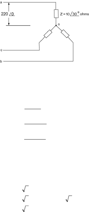
Figure 2.10 Load Connection for Example 2.2.

Solution

A. The phase currents are obtained as

A9011

3020

120220

A21011

3020

240220

A3011

3020

220

$

∠=

∠

=

∠=

∠

=

−∠=

∠

=

cn

bn

an

I

B. The line-to-line voltages are obtained as

$

2103220

903220120303220

303220

2402200220

−∠=

−∠=−∠=

∠=

∠−∠=

−=

ca

bc

bnanab

V

VVV

C. The apparent power into phase a is given by

VA302420

30)11)(220(

*

$

∠=

=

anana

IVS

The total apparent power is three times the phase value:

00.363035.6287

VA3000.72603032420

j

S

t

+=

∠=∠×=

$$

Thus

23

var00.3630

W35.6287

=

t

Q

P

Example 2.3

Repeat Example 2.2 as if the same three impedances were connected in a

∆

connection.

Solution

From Example 2.2 we have

$

2103220

903220

303220

−∠=

∠=

ca

bc

ab

V

The currents in each of the impedances are

$

120311

0311

3020

303220

∠=

−∠=

∠=

∠

=

ca

bc

ab

I

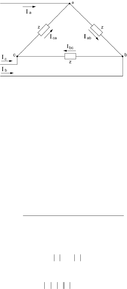
The line currents are obtained with reference to Figure 2.11 as

$

21033

9033

3033

1203110311

−∠=

−=

−∠=

−=

∠=

−∠−∠=

−=

bccac

abbcb

caaba

III

The apparent power in the impedance between a and b is

$

307260

)0322)(303220(

*

∠=

∠∠=

=

ababab

IVS

The total three-phase power is then

24

Figure 2.11 Load Connection for Example 2.3.

00.1089002.862,18

3021780

j

S

t

+=

∠=

$

As a result,

var00.21780

W04.37724

=

t

Q

P

2.4 THE PER UNIT SYSTEM

The per unit (p.u.) value representation of electrical variables in power

system problems is favored in electric power systems. The numerical per unit

value of any quantity is its ratio to a chosen base quantity of the same

dimension. Thus a per unit quantity is a normalized quantity with respect to the

chosen base value. The per unit value of a quantity is thus defined as

dimensionsamehteof valuebaseorReference

valueActual

valuep.u.

=

(2.25)

Five quantities are involved in the calculations. These are the current I,

the voltage V, the complex power S, the impedance Z, and the phase angles. The

angles are dimensionless; the other four quantities are completely described by

knowledge of only two of them. An arbitrary choice of two base quantities will

fix the other base quantities. Let

b

I

and

b

V

represent the base current and

base voltage expressed in kiloamperes and kilovolts, respectively. The product

of the two gives the base complex power in megavoltamperes (MVA)

MVA

bbb

IVS

=

(2.26)

25

The base impedance will also be given by

ohms

2

b

S

V

I

V

Z

==

(2.27)

The base admittance will naturally be the inverse of the base impedance. Thus,

siemens

1

2

b

V

S

V

I

Z

Y

=

==

(2.28)

The nominal voltage of lines and equipment is almost always known as

well as the apparent (complex) power in megavoltamperes, so these two

quantities are usually chosen for base value calculation. The same

megavoltampere base is used in all parts of a given system. One base voltage is

chosen; all other base voltages must then be related to the one chosen by the

turns ratios of the connecting transformers.

From the definition of per unit impedance, we can express the ohmic

impedance Z

Ω

in the per unit value Z

p.u

. as

p.u.

2

p.u.

b

V

SZ

Z

Ω

=

(2.29)

As for admittances, we have

p.u.

1

22

p.u.

b

S

b

S

V

Y

SZ

V

Z

Y

===

Ω

∆

(2.30)

Note that Z

p.u

. can be interpreted as the ratio of the voltage drop across

Z with base current injected to the base voltage.

Example 2.4

Consider a transmission line with

Ω+=

299.77346.3 jZ

. Assume that

kV735

MVA100

=

b

V

S

We thus have

26

()

Ω

−

ΩΩ

×=

⋅=⋅=

Z

V

S

ZZ

b

4

22

p.u.

1085108.1

)735(

1000

For R = 3.346 ohms we obtain

(

)

44

p.u.

1019372.61085108.1)346.3(

−−

×=×=

R

For X = 77.299 ohms, we obtain

(

)

24

p.u.

10430867.11085108.1)299.77(

−−

×=×=

X

For the admittance we have

()

S

b

S

Y

S

V

YY

3

2

p.u.

1040225.5

100

735

×=

=

⋅=

For Y = 1.106065

×

10

-3

siemens, we obtain

(

)

(

)

97524.5

10106065.11040225.5

33

p.u.

=

××=

−

Y

Base Conversions

Given an impedance in per unit on a given base

0

b

S

and

0

b

V

, it is sometimes

required to obtain the per unit value referred to a new base set

n

b

S

and

n

b

V

.

The conversion expression is obtained as:

2

p.u.p.u.

0

n

b

V

S

ZZ

⋅=

(2.31)

which is our required conversion formula. The admittance case simply follows

the inverse rule. Thus,

27

2

p.u.p.u.

0

b

V

S

YY

n

⋅= (2.32)

Example 2.5

Convert the impedance and admittance values of Example 2.4 to the new base of

200 MVA and 345 kV.

Solution

We have

24

p.u.

10430867.11019372.6

0

−−

×+×=

jZ

for a 100-MVA, 735-kV base. With a new base of 200 MVA and 345 kV, we

have, using the impedance conversion formula,

0

p.u.

2

p.u.p.u.

0775.9

345

735

100

200

Z

ZZ

n

=













⋅













=

Thus,

p.u. 102989.1106224.5

13

p.u.

−−

×+×=

jZ

n

For the admittance we have

0

p.u.

2

p.u.p.u.

11016.0

735

345

200

100

Y

YY

n

=













⋅













=

Thus,

p.u. 65825.0

)11016.0)(97524.5(

n

p.u.

=

Y

2.5 ELECTROMAGNETISM AND ELECTROMECHANICAL

ENERGY CONVERSION

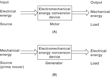
An electromechanical energy conversion device transfers energy between an

input side and an output side, as shown in Figure 2.12. In an electric motor, the

input is electrical energy drawn from the supply source and the output is

mechanical energy supplied to the load, which may be a pump, fan, hoist, or any

other mechanical load. An electric generator converts mechanical energy

28

Figure 2.12 Functional block diagram of electromechanical energy conversion devices as (A)

motor, and (B) generator.

supplied by a prime mover to electrical form at the output side. The operation of

electromechanical energy conversion devices is based on fundamental principles

resulting from experimental work.

Stationary electric charges produce electric fields. On the other hand,

magnetic field is associated with moving charges and thus electric currents are

sources of magnetic fields. A magnetic field is identified by a vector

B

called

the magnetic flux density. In the SI system of units, the unit of

B

is the tesla

(T). The magnetic flux

Φ

=

B

.

A

. The unit of magnetic flux

Φ

in the SI system

of units is the weber (Wb).

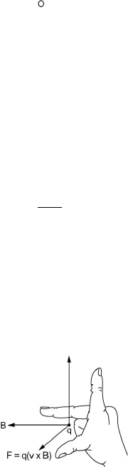
The Lorentz Force Law

A charged particle q, in motion at a velocity

V

in a magnetic field of

flux density

B

, is found experimentally to experience a force whose magnitude

is proportional to the product of the magnitude of the charge q, its velocity, and

the flux density

B

and to the sine of the angle between the vectors

V

and

B

and

is given by a vector in the direction of the cross product

V

×

B

. Thus we write

BVF

×=

q

(2.33)

Equation (2.33) is known as the Lorentz force equation. The direction

of the force is perpendicular to the plane of

V

and

B

and follows the right-hand

rule. An interpretation of Eq. (2.33) is given in Figure 2.13.

The tesla can then be defined as the magnetic flux density that exists

when a charge q of 1 coulomb, moving normal to the field at a velocity of 1 m/s,

experiences a force of 1 newton.

A distribution of charge experiences a differential force d

F

on each

29

moving incremental charge element dq given by

) (

BVF

×=

dqd

Moving charges over a line constitute a line current and thus we have

dlBF

) (

×=

Id

(2.34)

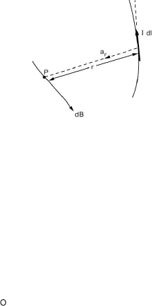
Equation (2.34) simply states that a current element I

dl

in a magnetic field

B

will experience a force d

F

given by the cross product of I

dl

and

B

. A pictorial

presentation of Eq. (2.34) is given in Figure 2.14.

The current element I

dl

cannot exist by itself and must be a part of a

complete circuit. The force on an entire loop can be obtained by integrating the

current element

∫

×=

BdlF

I

(2.35)

Equations (2.34) and (2.35) are fundamental in the analysis and design of

electric motors, as will be seen later.

The Biot-Savart law is based on Ampère’s work showing that electric

currents exert forces on each other and that a magnet could be replaced by an

equivalent current.

Consider a long straight wire carrying a current I as shown in Figure

2.15. Application of the Biot-Savart law allows us to find the total field at P as:

R

I

π

µ

2

B

0

= (2.36)

The constant

µ

0

is called the permeability of free space and in SI units is given

by

-7

0

10 4

×=

πµ

The magnetic field is in the form of concentric circles about the wire,

Figure 2.13 Lorentz force law.

30

Figure 2.14 Interpreting the Biot-Savart law.

with a magnitude that increases in proportion to the current I and decreases as

the distance from the wire is increased.

The Biot-Savart law provides us with a relation between current and the

resulting magnetic flux density

B

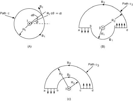
. An alternative to this relation is Ampère’s

circuital law, which states that the line integral of

B

about any closed path in

free space is exactly equal to the current enclosed by that path times

µ

0

.







=⋅

∫

Ic

IcI

c

enclosenotdoespath0

enclosespath

0

µ

dlB

(2.37)

It should be noted that the path c can be arbitrarily shaped closed loop about the

net current I.

2.6 PERMEABILITY AND MAGNETIC FIELD INTENSITY

To extend magnetic field laws to materials that exhibit a linear

variation of

B

with I, all expressions are valid provided that

µ

0

is replaced by the

permeability corresponding to the material considered. From a

B

-I – variation

point of view we divide materials into two classes:

1. Nonmagnetic material such as all dielectrics and metals with

permeability equal to

µ

0

for all practical purposes.

2. Magnetic material such as ferromagnetic material (the iron

group), where a given current produces a much larger

B

field

than in free space. The permeability in this case is much

higher than that of free space and varies with current in a

nonlinear manner over a wide range. Ferromagnetic material

can be further categorized into two classes:

a) Soft ferromagnetic material for which a linearization of

the

B

-I variation in a region is possible. The source of

B

in the case of soft ferromagnetic material can be modeled

as due to the current I.

b) Hard ferromagnetic material for which it is difficult to

31

Figure 2.15 Illustrating Ampère’s circuital law: (A) path c

1

is a circle enclosing current I, (B) path

c

2

is not a circle but encloses current I, and (C) path c

3

does not enclose current I.

give a meaning to the term permeability. Material in

this group is suitable for permanent magnets.

For hard ferromagnetic material, the source of

B

is a combined effect of

current I and material magnetization M, which originates entirely in the medium.

To separate the two sources of the magnetic

B

field, the concept of magnetic

field intensity

H

is introduced.

Magnetic Field Intensity

The magnetic field intensity (or strength) denoted by

H

is a vector

defined by the relation

HB

µ

= (2.38)

For isotropic media (having the same properties in all directions),

µ

is a scalar

and thus

B

and

H

are in the same direction. On the basis of Eq. (2.38), we can

write the statement of Ampère’s circuital law as

∫







=⋅

Ic

IcI

enclosenotdoespath0

enclosespath

dlH

(2.39)

The expression in Eq. (2.39) is independent of the medium and relates the

magnetic field intensity

H

to the current causing it, I.

Permeability

µ

is not a constant in general but is dependent on

H

and,

strictly speaking, one should state this dependence in the form

El-Hawary M.E. Electrical Energy Systems

Подождите немного. Документ загружается.