Coburn J.W. Algebra and Trigonometry
Подождите немного. Документ загружается.


EXERCISES
Solve using elimination. If a system is inconsistent or dependent, so state. For systems with linear dependence, give
the answer as an ordered triple using a parameter.
11. 12. 13.
Solve using a system of three equations in three variables.
14. In one version of the card game Gin Rummy, numbered cards (N) 2 through 9 are worth 5 points, the 10s and all
face cards (F) are worth 10 points, and aces (A) are worth 20 points. At the moment his opponent said “Gin!”
Kenan had 12 cards in his hand, worth a total value of 125 points. If the value of his aces and face cards was
equal to four times the value of his numbered cards, how many aces, face cards, and numbered cards was he
holding?
15. A vending machine accepts nickels, dimes, and quarters. At the end of a week, there is a total of $536 in the
machine. The number of nickels and dimes combined is 360 more than the number of quarters. The number of
quarters is 110 more than twice the number of nickels. How many of each type of coin are in the machine?
SECTION 8.3 Nonlinear Systems of Equations and Inequalities
KEY CONCEPTS
•
Nonlinear systems of equations can be solved using substitution or elimination.
•
First identify the graphs of the equations in the system to help determine the number of solutions possible.
•
For nonlinear systems of inequalities, graph the related equation for each inequality given, then use a test point to
decide what region to shade as the solution.
•
The solution for the system is the overlapping region (if it exists) created by solutions to the individual inequalities.
•
If the boundary is included, graph it using a solid line; if the boundary is not included use a dashed line.
EXERCISES
Solve Exercises 16–21 using substitution or elimination. Identify the graph of each relation before you begin.
16. 17. 18.
19. 20. 21.
SECTION 8.4 Systems of Linear Inequalities and Linear Programming
KEY CONCEPTS
•
As in Section 8.3, to solve a system of linear inequalities, we find the intersecting or overlapping areas of the
solution regions from the individual inequalities. The common area is called the feasible region.
•
The process known as linear programming seeks to maximize or minimize the value of a given quantity under
certain constraints or restrictions.
•
The quantity we attempt to maximize or minimize is called the objective function.
•
The solution(s) to a linear programming problem occur at one of the corner points of the feasible region.
•
The process of solving a linear programming application contains these six steps:
•
Identify the main objective and the decision variables.
•
Write the objective function in terms of these variables.
•
Organize all information in a table, using the decision variables and constraints.
•
Fill in the table with the information given and write the constraint inequalities.
•
Graph the constraint inequalities and determine the feasible region.
•
Identify all corner points of the feasible region and test these points in the objective function.
e
x
2
y
2
7 9
x
2
y 3
e
y x
2
2
x
2
y
2
16
e
x
2
y
2
10
y 3x
2
0
e
x
2
y 1
x
2
y
2
7
e
x y
2
1
x 4y 5
e
x
2
y
2
25
y x 1
•
3x y 2z 3
x 2y 3z 1
4x 8y 12z 7
•
x y 2z 2
x y z 1
2x y z 4
•
x y 2z 1
4x y 3z 3
3x 2y z 4
840 CHAPTER 8 Systems of Equations and Inequalities 8-48
College Algebra & Trignometry—
cob19529_ch08_793-846.qxd 11/28/08 16:06 Page 840
8-49 Mixed Review 841
EXERCISES
Graph the solution region for each system of linear inequalities and verify the solution using a test point.
22. 23. 24.
25. Carefully graph the feasible region for the system of inequalities
shown, then maximize the objective function:
26. After retiring, Oliver and Lisa Douglas buy and work a small farm (near Hooterville) that consists mostly of milk
cows and egg-laying chickens. Although the price of a commodity is rarely stable, suppose that milk sales bring
in an average of $85 per cow and egg sales an average of $50 per chicken over a period of time. During this time
period, the new ranchers estimate that care and feeding of the animals took about 3 hr per cow and 2 hr per
chicken, while maintaining the related equipment took 2 hr per cow and 1 hr per chicken. How many animals of
each type should be maintained in order to maximize profits, if at most 1000 hr can be spent on care and feeding,
and at most 525 hr on equipment maintenance?
e
x 2y 1
2x y 2
e
x 4y 5
x 2y 0
e
x y 7 2
x y 6 4
MIXED REVIEW
1. Write the equations in each system in slope-intercept
form, then state whether the system is
consistent/independent, consistent/dependent, or
inconsistent. Do not solve.
a. b.
c.
2. Solve by graphing. 3. Solve using a substitution.
4. Solve using elimination.
5. A burrito stand sells a veggie burrito for $2.45 and a
beef burrito for $2.95. If the stand sold 54 burritos in
one day, for a total revenue of $148.80, how many of
each did they sell?
Solve using elimination.
6.
7. •
0.1x 0.2y
z 1.7
0.3x
y 0.1z 3.6
0.2x 0.1y 0.2z 1.7
•
x 2y 3z 4
3x 4y z 1
2x 6y z 1
e
7x 4y 5
3x 2y 9
e
2x 3y 5
x 5y 17
e
x 2y 6
2x y 9
e
x 3y 9
6y 2x 10
e
4x 3y 9
2x 5y 10
e
3x 5y 10
6x 20 10y
Solve using elimination. If the system has coincident
dependence, state the solution set using set notation.
8. 9.
10. It’s the end of another big day at the circus, and the
clowns are putting away their riding equipment—a
motley collection of unicycles, bicycles, and tricycles.
As she loads them into the storage shed, Trixie counts
21 cycles in all with a total of 40 wheels. In addition,
she notes the number of bicycles is one fewer than
twice the number of tricycles. How many cycles of
each type do the clowns use?
Solve each system of inequalities by graphing the
solution region.
11. 12.
13.
14. Graph the solution region for the system of
inequalities. μ
4x 2y 14
2x 3y 15
y 0
x 0
e
x 2y 5
x 2y
e
2x y 6 3
2x y 7 3
e
2x y 4
x 3y 7 6
•
x 2y 3z 4
2x y z 1
5x z 6
•
x 2y 3z 4
2x y z 1
5x z 2
x y 7
2x y 10
2x 3y 18
x 0, y 0
f 1x, y2 30x 45y
⎞
⎪
⎬
⎪
⎠
College Algebra & Trignometry—
cob19529_ch08_839-846.qxd 12/1/08 4:55 PM Page 841 epg HD 049 :Desktop Folder:Satya 01/12/08:

15. Maximize given
16. Solve the system by substitution.
e
x
2
y
2
1
x y 1
μ
x y 8
x 2y 14
4x 3y 30
x, y 0
P1x, y2 2.5x 3.75y,
17. Solve using elimination:
18. Solve using the method of your choice.
Solve each system of inequalities.
19. 20. e
x
2
y
2
6 4
x
2
y
6 0
e
x y 7 1
x
2
y
2
16
e
y 1 x
2
x
2
y 7
e
4x
2
y
2
9
x
2
3y
2
79
842 CHAPTER 8 Systems of Equations and Inequalities 8-50
PRACTICE TEST
Solve each system and state whether the system is
consistent, inconsistent, or dependent.
1. Solve graphically: 2. Solve using substitution:
3. Solve using elimination: 4. Solve using elimination:
5. Solve using elimination:
6. Find values of a and b such that is a solution
of the system.
Create a system of equations to model each exercise,
then solve using the method of your choice.
7. The perimeter of a “legal-size” paper is 114.3 cm.
The length of the paper is 7.62 cm less than twice
the width. Find the dimensions of a legal-size sheet
of paper.
8. The island nations of Tahiti and Tonga have a
combined land area of 692 mi
2
. Tahiti’s land area is
112 mi
2
more than Tonga’s. What is the land area of
each island group?
9. Many years ago, two cans of corn (C), 3 cans of
green beans (B), and 1 can of peas (P) cost $1.39.
Three cans of C, 2 of B, and 2 of P cost $1.73. One
e
ax by 12
bx ay 1
12, 12
•
2x y z 4
x 2z 1
x 2y 8z 11
•
x 2y z 4
2x 3y 5z 27
5x y 4z 27
e
5x 8y 1
3x 7y 5
e
3x y 2
7x 4y 6
e
3x 2y 12
x 4y 10
can of C, 4 of B, and 3 of P cost $1.92. What was the
price of a single can of C, B, and P?
10. After inheriting $30,000 from a rich aunt, David
decides to place the money in three different
investments: a savings account paying 5%, a bond
account paying 7%, and a stock account paying 9%.
After 1 yr he earned $2080 in interest. Find how
much was invested at each rate if $8000 less was
invested at 9% than at 7%.
11. Solve the system of inequalities by graphing.
12. Maximize the objective function:
Solve the linear programming problem.
13. A company manufactures two types of T-shirts, a
plain T-shirt and a deluxe monogrammed T-shirt. To
produce a plain shirt requires 1 hr of working time
on machine A and 2 hr on machine B. To produce a
deluxe shirt requires 1 hr on machine A and 3 hr on
machine B. Machine A is available for at most
50 hr/week, while machine B is available for at most
120 hr/week. If a plain shirt can be sold at a profit of
$4.25 each and a deluxe shirt can be sold at a profit
of $5.00 each, how many of each should be
manufactured to maximize the profit?
Solve each nonlinear system using the technique of
your choice.
14. 15. e
4y x
2
1
y
2
x
2
4
e
x
2
y
2
16
y x 2
•
x 2y 8
8x 5y 40
x, y 0
P 50x 12y
e
x y 2
x 2y 8
College Algebra & Trignometry—
cob19529_ch08_793-846.qxd 11/28/08 16:07 Page 842
8-51 Calculator Exploration and Discovery 843
16. A support bracket on the frame of a large ship is a
steel right triangle with a hypotenuse of 25 ft and a
perimeter of 60 ft. Find the lengths of the other sides
using a system of nonlinear equations.
17. Solve .
18. Write a system of inequalities that describes all
the points with positive y-values that are less than
3 units away from the origin.
e
x
2
y 2
x y
2
2
19. Solve the system of
inequalities.
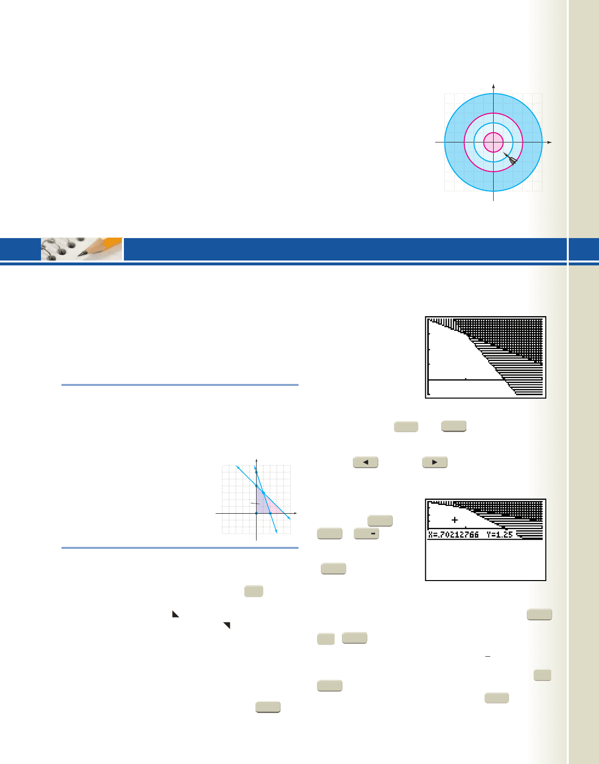
20. Write a system of
four inequalities that
describes the
location of the dart
on the dartboard
shown.
•
2x y 1
3x 2y 2
x 3y 3
543215 4 3 2 1
1
2
3
4
5
2
3
4
5
1
yy
xx
CALCULATOR EXPLORATION AND DISCOVERY
Optimal Solutions and Linear Programming
In this exercise, we’ll use a graphing calculator to explore
various areas of the feasible region, repeatedly evaluating
the objective function to see where the maximal values
(optimal solutions) seem to “congregate.” If all goes as
expected, ordered pairs nearest to a vertex should give rel-
atively larger values. To demonstrate, we’ll use Example
6 from Section 8.4, stated below.
Example 6
Find the maximum value of the objective
function given the constraints shown:
.
Solution
The feasible region is
shown in lavender. There are four
corner points to this region: (0, 0),
(0, 4), (2, 0), and (1, 3), and we
found f(x, y) was maximized at
(1, 3): .
To explore this feasible region in terms of the objec-
tive function enter the boundary lines
and on the screen.
However, instead of shading below the lines to show the
feasible region (using the feature to the extreme left),
we shade above both lines (using the feature) so that
the feasible region remains clear. Setting the window size
at and produces Figure 8.22.
Using will leave a blank area just below
QI that enables you to explore the feasible region as the
x- and y-values are displayed. Next we place the calcula-
tor in “split-screen” mode so that we can view the graph
and the home screen simultaneously. Press the key
MODE
YMin 1.5
y 31.5, 44x 30, 34
Y =
Y
2
3x 6Y
1
x 4
f 1x, y2 2x y,
f 11, 32 5
μ
x y 4
3x y 6
x 0
y 0
f 1x, y2 2x y
and notice the second-
to-last line reads Full
Horiz G-T. The Full
(screen) mode is the
default operating
mode. The Horiz
mode splits the screen
horizontally, placing
the graph directly
above a shorter home
screen. Highlight
Horiz, then press and to have the calcula-
tor reset the screen in this mode. The TI-84 Plus has a
free-moving cursor that is brought into view by pressing
the left or right arrow (Figure 8.23). A
useful feature of this
cursor is that it auto-
matically stores the
current X value as the
variable X ( or
) and
the current Y value
as the variable Y
( 1), which
allows us to evaluate
the objective function
right on the home screen. To access the
graph and free-moving cursor you must press
each time, and to access the home screen you must press
(QUIT) each time. Begin by moving the
cursor to the upper-left corner of the region, near the
y-intercept [we stopped at (~0.0957, . Once you
have the cursor “tucked up into the corner,” press
(QUIT) to get to the home screen, then enter the
objective function: . Pressing evaluates
the function for the values indicated by the cursor’s location
ENTER
2X Y
MODE
2nd
3.2624
MODE
2nd
GRAPH
f 1x, y2 2x y
ALPHA
STO
ALPHA
X,T,,n
GRAPH
ENTER
55
3
7
y
x
(1, 3)
(0, 6)
Feasible
region
Exercise 20
4
03
1.5
4
03
1.5
Figure 8.22
Figure 8.23
College Algebra & Trignometry—
cob19529_ch08_793-846.qxd 11/28/08 16:07 Page 843
844 CHAPTER 8 Systems of Equations and Inequalities 8-52
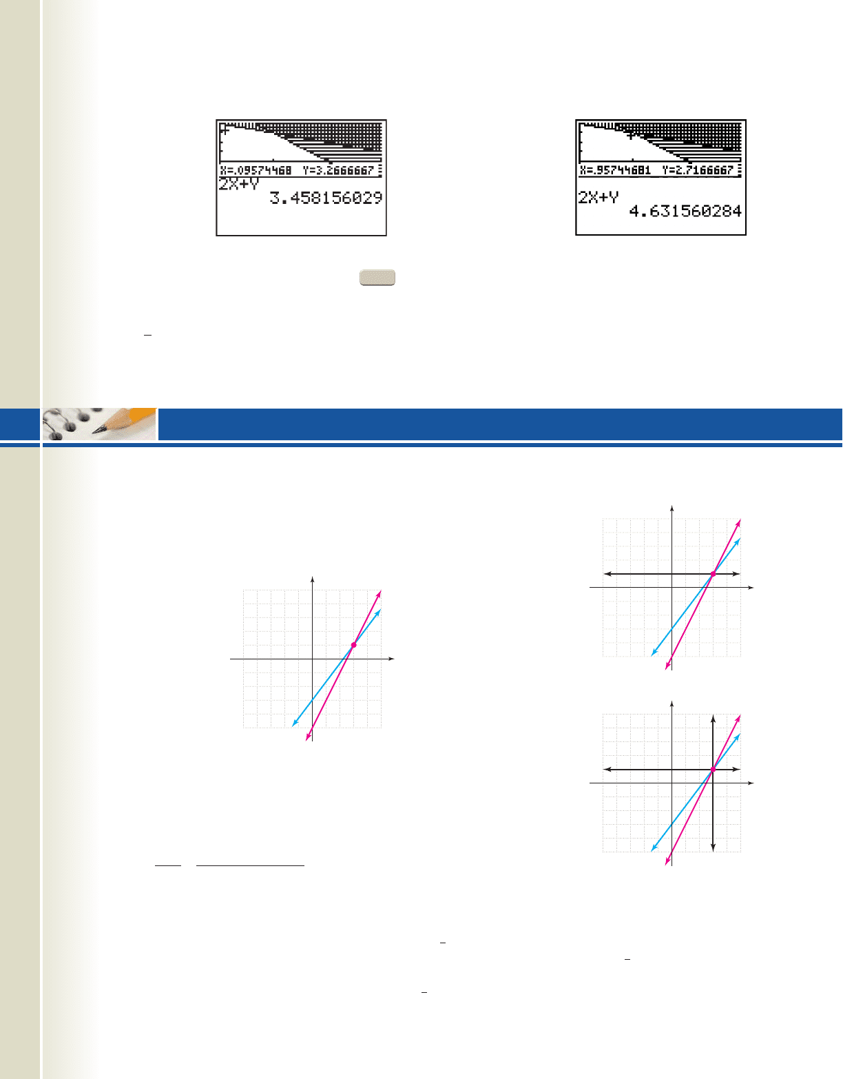
(Figure 8.24). It
appears the value of
the objective function
for points (x, y) in this
corner are close to 4,
and it’s no accident
that at the corner
point (0, 4) the
maximum value is in
fact 4. Repeating this
procedure for the lower-right corner suggests the
maximum value near (2, 0) is also 4. Finally, press
to explore the region in the upper-right corner, where the
lines intersect. Move the cursor to this vicinity, locate it
very near the point of intersection [we stopped at
( and return to the home screen and eval-
uate (Figure 8.25). The value of the objective function is
0.957, 2.71624
GRAPH
near 5 in this corner of
the region, and at the
corner point (1, 3) the
maximum value is 5.
Exercise 1: The feasi-
ble region for the
system given to the
right has four corner
points. Use the ideas
here to explore the area
near each corner point of the feasi-
ble region to determine which point
is the likely candidate to produce
the minimum value of the objective
function Then
solve the linear programming
problem to verify your guess.
f 1x, y2 2x 4y.
When asked to solve a system of two equations in two
variables, we first select an appropriate method. In
Section 8.1, we learned three basic techniques: graphing,
substitution, and elimination. In this feature, we’ll explore
how these methods are
related using Example 2
from Section 8.1 where we
were asked to solve the
system
by graphing. The result-
ing graph, shown here in
Figure 8.26, clearly indi-
cates the solution is (3, 1).
As for the elimination
method, either x or y can be
easily eliminated. If the second equation is multiplied by
2, the x-coefficients will be additive inverses, and the sum
results in an equation with y as the only unknown.
The result is but remember, this is a system
of linear equations, and is still the equation of a
(horizontal) line. Since the system is equi-
valent to the original, it will have the same solution set. In
Figure 8.27, we note the point of intersection for the new
system is still (3, 1). If we eliminate the y-terms instead
e
4x 3y 9
y 1
y 1
y 1
R1 4x 3y 9
2R2 4x 2y 10
sum y 1
e
4x 3y 9
2x
y 5
(using , the
result is , which is
also the equation of a (ver-
tical) line. Creating another
equivalent system using
this line produces
and the graph shown in
Figure 8.28, where the
vertical and horizontal
lines intersect at (3, 1),
making the solution trivial.
Note: Here we see a
close connection to solving
general equations, in that
the goal is to write a series
of equivalent yet simpler
equations, continuing until
the solution is obvious.
As for the substitution
method, consider the
second equation written as
. This equation
represents every point (x, y) on its graph, meaning the rela-
tionship for the ordered pair solutions can also be written
. The same thing can be said for the line
, with its ordered pair solutions represented by
. At the point of intersection the y-coordinates
must be identical, giving . In other words,
we can substitute for y in the first equation, or
for y in the second equation, with both yielding the
4
3
x 3
2x 5
2x 5
4
3
x 3
1x,
4
3
x 32
4x 3y 9
1x, 2x 52
y 2x 5
e
x 3
y 1
x 3
R1 3R22
4
03
1.5
Figure 8.24
4
03
1.5
Figure 8.25
μ
2x 2y 15
x y 6
x 4y 9
x, y 0
Understanding Why Elimination and Substitution “Work”
x
y
543215 4 3 2 1
5
4
3
2
1
5
4
3
2
1
(3, 1)
x
y
543215 4 3 2 1
5
4
3
2
1
5
4
3
2
1
x
y
543215 4 3 2 1
5
4
3
2
1
5
4
3
2
1
Figure 8.26
Figure 8.27
Figure 8.28
College Algebra & Trignometry—
STRENGTHENING CORE SKILLS
cob19529_ch08_793-846.qxd 11/28/08 16:07 Page 844
8-53 Cumulative Review Chapters 1–8 845
correct solution. Substituting for y in the first equa-
tion gives
substitute for y
expand
simplify
and the solution becomes or (3, 1).13, 2132 521x, 2x 52
x 3
2x 6
4 x 6x 15 9
2x 5 4 x 312x 52 9
2x 5
All three methods will produce the same solution,
and the best method to use at the time often depends on
the nature of the system given, or even personal
preference.
Exercise 1: Solve the system by
(a) graphing, (b) elimination, and
(c) substitution. Which method was
most efficient for solving this system?
CUMULATIVE REVIEW CHAPTERS 1–8
Graph each of the following. Include x- and y-intercepts
and other important features of each graph.
1. 2.
3. 4.
5.
6.
7.
8.
9. Graph Give the coordinates of all
intercepts and the equation of all asymptotes.
10. Chance’s skill at bowling is slowly improving with
practice. In February his average score was 102, but
by May he had raised his average to 126. Assuming
the relationship is linear, (a) find the equation of the
line, (b) explain what the slope of the line means in
this context, and (c) predict the month when
Chance’s average score will exceed 151.
11. Determine the following for
the graph shown to the right.
Use interval notation as
appropriate.
a. domain
b. range
c. interval(s) where f(x) is
increasing or decreasing
d. interval(s) where f(x) is constant
e. location of any maximum or minimum value(s)
f. interval(s) where f(x) is positive or negative
g. the average rate of change using and
12, 3.52.
14, 02
h1x2
9 x
2
x
2
4
.
y tana2x
2
b
y 2 sinax
4
b
y 2
x
3
g1x2 1x 321x 121x 42
h1x2
1
x 1
2g1x2 1x 3 1
f 1x2
x 2
3y
2
3
x 2
12. Suppose the cost of making a rubber ball is given by
where x is the number of balls in
hundreds. If the revenue from the sale of these balls
is given by find the
profit function How
many balls should be produced and sold to obtain
the maximum profit? What is this maximum profit?
13. Solve each equation.
a.
b.
c.
d.
e.
f.
g.
h.
i.
Given and find:
14. Solve each equation in
a.
b.
15. Solve using a special triangle.
16. Solve using trigonometric
ratios (round to tenths).
A
__
, B 63°, C 90°
a
__
, b
__
, c 82
A 30°, B
__
, C 90°
a 20, b
__
, c
__
3 tanax
4
b 713
413
2 sin12x2 13 213
30, 22.
g1x2 3x
2
2xf1x2 2x 5
log
3
x log
3
1x 22 1
log
3
81 x
3
x2
7
4
#
2
x1
1
8
x
2
3x
1
40 0
x
2
6x 13 0
2
n 4
3 13
x
3
2
8 0
1x
2 13x 4
1Profit Revenue Cost2.
R1x2x
2
123x 1990,
C1x2 3x 10,
e
2x y 2
4x 3y 8
4321
1
6 45 321
1
2
3
4
5
2
3
4
1
x
y
(0, 3.5)
5
C
A
B
20 m
30
CA
B
82 ft
63
College Algebra & Trignometry—
cob19529_ch08_839-846.qxd 12/30/08 22:42 Page 845
26.
Solve each system using elimination.
27.
28.
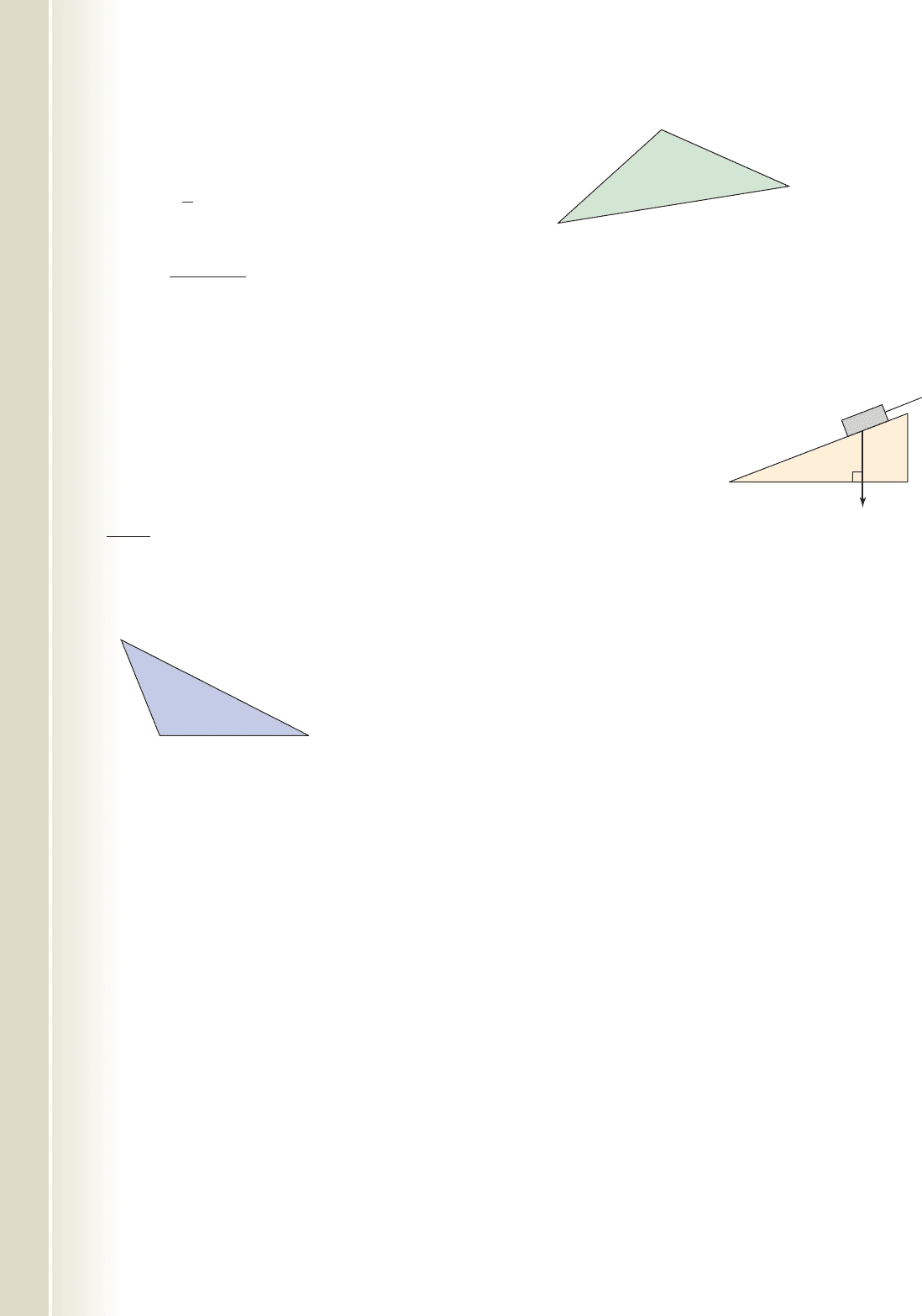
29. A 900-lb crate is
sitting on a ramp that
has a incline. Find
the force needed to
hold the crate
stationary.
30. A jet plane is flying at 750 mph on a heading of
There is a strong, 50 mph wind blowing from due
south (heading ). What is the true course and
speed of the plane (relative to the ground)?
0°
30°.
28°
•
x 2y z 0
2x 5y 4z 6
x 3y 4z 5
e
4x 3y 13
9x 5y 6
C
A
B
31 cm
52 cm
33
17. State the three Pythagorean identities.
18. Find in Quadrant IV given
19. State the value of all six trig functions given
with
20. Verify the following is an identity:
21. Find the average rate of change in the interval
[1.1, 1.2] for
22. Use the rational roots theorem to factor the
polynomial completely:
.
Solve each inequality. Write your answer using interval
notation.
23.
24.
Solve each triangle using either the law of sines or the
law of cosines, whichever is appropriate.
25.
C
A
B
19 in.
112
41
x 2
x 3
3
x
2
3x 10 6 0
x
4
6x
3
13x
2
24x 36
f1x2 x
2
3x.
tan
4
1 sec
2
1 csc
2
cos 7 0.tan
3
4
r
32°.
G
21
900 lb
College Algebra & Trignometry—
846
CHAPTER 8 Systems of Equations and Inequalities 8-54
cob19529_ch08_839-846.qxd 12/1/08 4:55 PM Page 846 epg HD 049 :Desktop Folder:Satya 01/12/08:

Matrices and Matrix
Applications
CHAPTER OUTLINE
9.1 Solving Linear Systems
Using Matrices and Row Operations 848
9.2 The Algebra of Matrices 859
9.3 Solving Linear Systems
Using Matrix Equations 872
9.4 Applications of Matrices and Determinants:
Cramer’s Rule, Partial Fractions, and More 886
9
9
CHAPTER CONNECTIONS
From pediatric and geriatric care, to the training
of a modern athlete, dietetic applications have
become increasingly effective. In the latter
case, athletes generally need high levels of
carbohydrates and protein, but only moderate
levels of fat. Suppose a physical trainer wants
to supply one of her clients with 24 g of fat,
244 g of “carbs,” and 40 g of protein for the
noontime meal. Knowing the amount of these
nutrients contained in certain foods, the trainer
can recommend a variety of foods and the
amount of each that should be eaten. The
matrix operations in this chapter demonstrate
how to do this effectively. This application
occurs as Exercise 78 in Section 9.3.
Check out these other real-world connections:
Calculating Contract Totals for Home
Improvement Jobs (Section 9.2, Exercise 61)
Calculating Appropriate Resource Allocation
(Section 9.3, Exercise 71)
Applying the Mean Value Principle of Physics
and Thermal Conductivity
(Section 9.3, Exercise 73)
Calculating Area of Norman Windows
(Section 9.4, Exercise 49)
847
College Algebra & Trignometry—
cob19529_ch09_847-858.qxd 12/1/08 4:25 PM Page 847 epg HD 049 :Desktop Folder:Satya 01/12/08:

9.1 Solving Linear Systems Using Matrices and Row Operations
Just as synthetic division streamlines the process of polynomial division, matrices and
row operations streamline the process of solving systems using elimination. With the
equations of the system in standard form, the location of the variable terms and
constant terms are set, and we simply apply the elimination process on the coefficients
and constants.
A. Introduction to Matrices
In general terms, a matrix is simply a rectangular arrangement of numbers, called
the entries of the matrix. Matrices (plural of matrix) are denoted by enclosing the
entries between a left and right bracket, and named using a capital letter, such as
and They occur in many different sizes B £
2 13
462
101
§.A c
1 32
511
d
848 9-2
Learning Objectives
In Section 9.1 you will learn how to:
A. State the size of a
matrix and identify its
entries
B. Form the augmented
matrix of a system of
equations
C. Solve a system of
equations using row
operations
D. Recognize inconsistent
and dependent systems
E. Solve applications using
linear systems
as defined by the number of rows and columns each has, with the number of rows
always given first. Matrix A is said to be a 2 3 (two by three) matrix, since it has two
rows and three columns. Matrix B is a 3 3 (three by three) matrix.
EXAMPLE 1A
Identifying the Size and Entries of a Matrix
Determine the size of each matrix and identify the entry located in the second row
and first column.
a. b.
Solution
a. Matrix C is 3 2. The row 2, column 1 entry is 1.
b. Matrix D is 3 4. The row 2, column 1 entry is 0.4.
If a matrix has the same number of rows and columns, it’s called a square matrix.
Matrix B above is a square matrix, while matrix Ais not. For square matrices, the values
on a diagonal line from the upper left to the lower right are called the diagonal entries
and are said to be on the diagonal of the matrix. When solving systems using matri-
ces, much of our focus is on these diagonal entries.
EXAMPLE 1B
Identifying the Diagonal Entries of a Square Matrix
Name the diagonal entries of each matrix.
a. b.
Solution
a. The diagonal entries of matrix E are 1 and 3.
b. For matrix F, the diagonal entries are 0.2, 0.3, and 0.6.
Now try Exercises 7 through 9
B. The Augmented Matrix of a System of Equations
A system of equations can be written in matrix form by augmenting or joining the coef-
ficient matrix, formed by the variable coefficients, with the matrix of constants.
F £
0.2 0.5 0.7
0.4 0.3 1
2.1 0.1 0.6
§E c
14
2 3
d
D £
0.2 0.5 0.7 3.3
0.4 0.3 1 2
2.1 0.1 0.6 4.1
§C £
3 2
15
43
§
A. You’ve just learned how
to state the size of a matrix
and identify its entries
College Algebra & Trignometry—
cob19529_ch09_847-858.qxd 12/1/08 4:25 PM Page 848 epg HD 049 :Desktop Folder:Satya 01/12/08:

9-3 Section 9.1 Solving Linear Systems Using Matrices and Row Operations 849
The coefficient matrix for the system is with
column 1 for the coefficients of x, column 2 for the coefficients of y, and so on. The
matrix of constants is These two are joined to form the augmented matrix,
with a dotted line often used to separate the two as shown here: .
It’s important to note the use of a zero placeholder for the y-variable in the second row
of the matrix, signifying there is no y-variable in the corresponding equation.
£
2311
10 12
1 345
§
£
1
2
5
§.
£
231
10 1
1 34
§•
2x 3y z 1
x
z 2
x 3y 4z 5
EXAMPLE 2
Forming Augmented Matrices
Form the augmented matrix for each system, and name the diagonal entries of each
coefficient matrix.
a. b. c.
Solution
a.
Diagonal entries: 2 and 3.
b.
Diagonal entries: 1, 5, and 3.
c.
Diagonal entries: and 1.
Now try Exercises 10 through 12
1
2
,
2
3
,
£
1
2
107
1
2
3
5
6
11
12
0 2 1 3
§
¡
•
1
2
x y
7
x
2
3
y
5
6
z
11
12
2y z 3
£
141 10
25 8 4
1 2 3 7
§
¡
•
x 4y z 10
2x 5y 8z 4
x 2y 3z 7
c
2111
132
d
¡
e
2x y 11
x 3y 2
•
1
2
x y
7
x
2
3
y
5
6
z
11
12
2y z 3
•
x 4y z 10
2x 5y 8z 4
x 2y 3z 7
e
2x y 11
x 3y 2
This process can easily be reversed to write a system of equations from a given
augmented matrix.
EXAMPLE 3
Writing the System Corresponding to an Augmented Matrix
Write the system of equations corresponding to each matrix.
a. b. £
141 10
0 310 7
00 1 1
§c
3 5 14
01 4
d
Solution
a.
b.
Now try Exercises 13 through 18
•
1x 4y 1z 10
0x 3y 10z 7
0x 0y 1z 1
¡
£
141 10
0 310 7
00 1 1
§
e
3x 5y 14
0x 1y 4
¡
c
3 5 14
01 4
d
B. You’ve just learned how
to form the augmented matrix
of a system of equations
College Algebra & Trignometry—
cob19529_ch09_847-858.qxd 12/2/08 8:50 PM Page 849 epg HD 049 :Desktop Folder:Satya 02/12/08:
