Chandrasekaran A. (ed.) Current Trends in X-Ray Crystallography

Подождите немного. Документ загружается.

Investigating Macromolecular Complexes in

Solution by Small Angle X-Ray Scattering

Cristiano Luis Pinto Oliveira

Department of Experimental Physics, Institute of Physics, University of São Paulo

Brazil

1. Introduction

Macromolecular complexes have a huge interest in molecular biology. The comprehension

of the biological processes in living systems is directly related to the knowledge of the shape

and structure of the formed complex and the process of formation. Although X-ray

diffraction, Nuclear Magnetic Resonance and cryoEM can provide information on the

formed structures, there are several cases where none of those techniques can be applicable.

Limitations on molecular weight, the necessity of a well ordered crystal, difficulties on

sample preparation etc, are some of the bottle necks of those techniques (Svergun, 2007;

Oliveira et al, 2010). Most importantly, in several cases the studies have to be performed

directly in solution, with minimum interaction with the studied sample in order to avoid

biased results. In this respect, scattering techniques are highly recommended since they

allow a study directly in solution in a very non-invasive way. Small angle X-Ray scattering

(SAXS) is a standard technique that can be applied to the study of particles in solution,

providing information on size, shape, polydispersity, flexibility, oligomerization and

aggregation state. Also, it allows real time measurements where the system can be

monitored directly in solution, enabling the study of the in situ particle formation (Oliveira

et al, 2009). The combination of SAXS and microscopy techniques has been used in several

applications due to their complementarity (Oliveira et al, 2010; Andersen et al, 2009). In this

chapter some general aspects of Small Angle X-Ray scattering and the state of the art

modeling methods will be presented, with several applications.

2. Small angle X-Ray scattering

When a collimated beam (assumed as parallel waves) of X-ray photons strikes a sample, a

fraction of the incident beam interacts with the electrons clouds of each molecule, and a

possible process is the absorption of this photon by the atoms which excites the electrons of

the atom to higher energy levels. When the excited electrons decay to ground state another

X-Ray photon is reemitted as a spherical wave. In this way, this process can be viewed as the

scattering of the incident photon over the electronic cloud. Depending on the energy of the

incident photon several processes can happen: Rayleigh scattering, Resonance scattering,

Compton effect, Thomson scattering, pair production, etc. It is beyond the scope of this

chapter investigate all these possible processes. However, under certain energy limits (~7-

12KeV), this scattering is well described by the so called first Born approximation, where the

Current Trends in X-Ray Crystallography

368

photon interacts only with one atom and the resulting scattered photon has the same energy

of the incident photon (elastic scattering). This effect is mostly related the so called Thomson

scattering. The complete solution of the scattered beam is a sum of a plane wave plus a

spherical wave (Jackson, 1988). Since the information of the scattering process is related with

the spherical wave only this part is considered to investigate the structural information of

the particle (Guinier and Fournet, 1955; Glatter and Kratky, 1982; Feigin and Svergun, 1987).

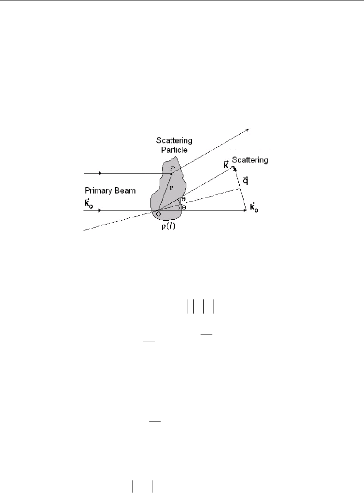
One possible way to understand the scattering process is to start from the concept of the

scattering from a single particle, fixed in space. This is sketched on Fig.1, where an incident

beam of wave vector



strikes the particle at the points O and P, separated by the vector r



Fig. 1. Representation of the scattering process for a fixed particle.

Since the scattering is assumed to be elastic, the scattered wave with wave vector



has the

same modulus of the incident wave so the difference between the incident and the scattered

beam is given by:

2sin

sin

qkk k k











 























(1)

which leads to the definition of the reciprocal space momentum transfer vector q. The

scattering amplitude







is given by the Fourier transformation of the particle electron

density









exp

rdr













(2)

The measurable quantity is the scattering intensity







, which is the square modulus of

the scattering amplitude:

   



 



exp

I q fq fq fq

I q r r r iq r drdr



















 

(3)

Investigating Macromolecular Complexes in Solution by Small Angle X-Ray Scattering

369

The index “1” indicates that until now this intensity is related to a single particle with fixed

orientation. One usual mathematical procedure is to take the convolution integral in r’ and

define as the so called self-correlation function





















rrrrdr















(4)

Now the scattering from a single fixed particle can be rewritten as,













exp

rdr











(5)

The self-correlation function









has several properties and asymptotic limits enabling the

retrieving of several general parameters. The interested reader is invited to read the seminal

book from Guinier and Fournet (Guinier and Fournet, 1955) and the articles from Ciccariello

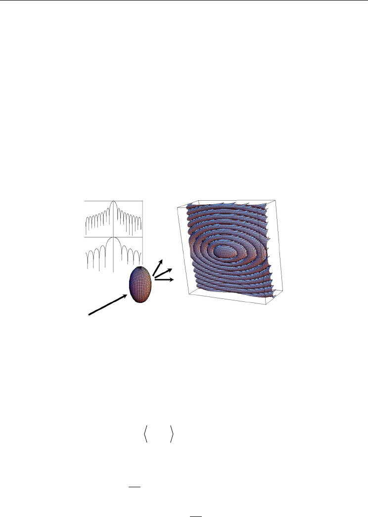
(Ciccariello, 1985) among others. A theoretical calculation of a 2D scattering profile for a

fixed particle in space is shown in Fig2.

Fig. 2. Theoretical calculation for a two dimensional scattering profile for a fixed ellipsoidal

particle. The intensity is given in logarithm scale. Inserts: vertical and horizontal 1D-profiles

of the intensity.

Equation (5) is still too general to be used in practice. In real systems, the particles

investigated are not fixed in space but instead they might be randomly oriented. The

averaging procedure can be made either in real space or in reciprocal space. From the

mathematical point of view is easier to perform the average in reciprocal space, by an extra

integration over the solid angle

:

 



qfq















(6)

Substituting (5) on (6) we have,



00 0

exp

Iq rdrd d r iqr

rdr rd iqrd





















 

 







(7)

Current Trends in X-Ray Crystallography

370

Where the volume integral element for dr



was written as

rdrd



, the spherical coordinates

in real space. In the last operation the terms were rearranged. The angular integrals can be

performed directly:







    

sin

exp

iq r

rrdrr











 











(8)

where the function







is known as average self-correlation function. With these

substitutions the intensity for a single particle randomly oriented is given by







sin

rrdr









(9)

The theoretical intensity of an ellipsoidal particle randomly oriented in space if shown in

Fig3. As can be directly seen, now the 2D spectra is angular independent and any cut

starting from the center towards a radial direction will have the same profile.

Fig. 3. Theoretical calculation for a two dimensional scattering profile for an ellipsoidal

particle randomly oriented. The intensity is given in logarithm scale. Insert: 1D-profiles of

the intensity.

One usual procedure is to define the so called pair distance distribution function p(r),









rrr



 which is a histogram of pair distances inside of the particle, weighted by the

distance length and by the product of the electron densities of the infinitesimal elements of

the pair (Glatter, 2002). The p(r) function permits the definition of the Fourier pair:









sin

Iq pr dr

rqIqdq









(10)

Investigating Macromolecular Complexes in Solution by Small Angle X-Ray Scattering

371

Some interpretations for the p(r) function will be explained in the next sections.

The result given in equation (10) was derived for a single particle randomly oriented in

space. In real systems the particles are dispersed in a matrix with electron density



and

therefore it is necessary to extrapolate this result for a system of particles. One expression

for the intensity of a system of particles is given by



() ()Iq N f q Sq



(11)

Where

 





is the so called particle form factor and the function

()Sq



is the

system structure factor. For systems composed of identical particles (monodisperse sytems)

the form factor is identical to the average scattering intensity of a single particle,











. For polydisperse systems the form factor will be an average over the different

sizes, electron densities and particle shapes. In this case, one usual procedure is to assume a

known shape and electron density and performs the average over a distribution of sizes

(Glatter and Kratky, 1982). On the other hand, the structure factor is related with particle

interactions and there are several approaches to describe its behavior (Pedersen, 2002). For

very diluted systems the particle interactions can be neglected and the structure factor is

equal to 1. Therefore for a system of identical particles in a dilute regime we have









 (12)

indicating that, although the measured intensity is a contribution of a large number of

particles, it contains the information of the scattering from a single particle randomly

oriented. This shows that in a real case where the intensity I(q) is measured, it might be

possible to obtain information about the single particle shape and conformation.

As mentioned above, the particles can be considered to be immersed in a matrix with

constant electron density. It can be shown that in this case the scattering event will only

happen if there are differences between the electron density of the particles and the matrix.

In this way the electron density



(r) shown in equations 2-5 should be replaced by the

electron density contrast



(r) =



(r)-



. In order to make this point clearer, one usual

approach is to consider the particle form factor to be normalized and the electronic mass is

explicitly shown:









Iq N VP q





(13)

where





, is the scattering contrast between the particles and the matrix, V is the

particle volume and P

(q) is the normalized form factor (P

(q=0)=1).

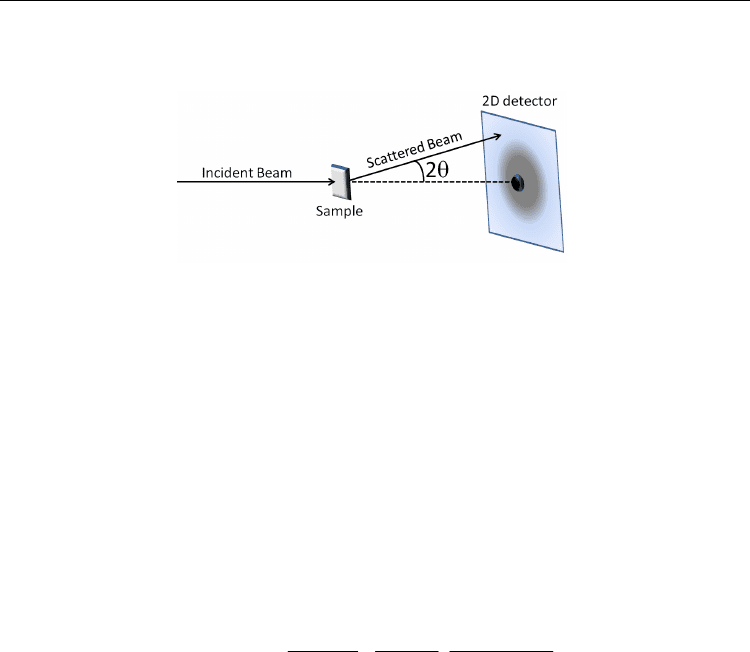
2.1 Experimental aspects and absolute calibration

A schematic setup for a typical SAXS experiment is shown in figure 4. Specific technical

details about geometries and configurations can be found in several sources (Lindner and

Zemb, 2002) and it will not be presented in this chapter. However, some general

characteristics have to be addressed. Since only a small fraction of the incident beam is

scattered, the detectors should be set to detect reasonably low intensities. Therefore the

incoming beam that passes without interaction with the sample has to be blocked by a beam

Current Trends in X-Ray Crystallography

372

stopper, to avoid possible damaging of the detector. The size of the beam stopper depends

on the equipment geometry.

Fig. 4. Schematic setup of a SAXS experiment.

In a typical experiment it is necessary to measure the intensity from the system (sample



matrix+particles) and subtract the intensity from the matrix where the particles are

immersed (blank). To normalize the data to absolute scale, scattering standards have to be

used. In the applications described in the present chapter two procedures were applied. In

one procedure a known protein is measured on the same sample conditions (buffer,

temperature, etc) and the forward scattering obtained for this sample is used to normalize

the other, unknown data. In other procedure water at 20ºC is used as primary standard. This

is a convenient standard since the value of the scattering cross section can be calculated with

very high accuracy from the fundamental macroscopic properties of water. In both cases, the

data has to be normalized by the value obtained from the standard on the same

experimental conditions and multiplied by the theoretical intensity value. Assuming that the

sample and the blank are measured in the same cell, the treated intensity, normalized to

absolute scale can be given by:













sample

blank

std

Treated

sss bbb

std

Tt Tt I













(14)

Where q is modulus of the scattering vector, defined as q = (4





) sin



, where 2



is the

scattering angle as shown in Fig1 and Fig4 and



is the wavelength of the monochromatic

beam; I

Treated

(q) is the treated scattering intensities for the sample on absolute scale, i.e. the

scattering cross section of the sample; I

sample

(q) is the raw data measured for the sample,

blank

(q) is the raw data from the matrix scattering; I(0)

std

is the value at q = 0 of treated

standard data (background subtracted and normalized by flux, transmission and acquisition

time);



is the flux of the incident beam; T

is the sample transmission and t

is the

exposure time, where the index i is s (sample), b (blank); (d





)

std

is the theoretical

scattering cross section for the standard. For water at 20ºC this cross section has the value

0.01632 [cm

-1

]. For proteins in typical buffers without high amounts of salt, glycerol or other

additives, the theoretical cross section for a system of proteins in solution with mass

concentration c (in mg/mL) and molecular weight M

(in kDa) is given by





)

std

=6.645x10

-4

c M

[cm

-1

] (see equation 15 below).

Having the data on absolute scale, information about its contrast, particle volume or particle

concentration can be obtained, depending on the knowledge about the system. One very

important parameter when studying proteins in solution is the determination of the

Investigating Macromolecular Complexes in Solution by Small Angle X-Ray Scattering

373

molecular weight, which is a direct indication of the oligomerization state of the protein.

Starting from equation (13), multiplying and dividing by the particle specific volume

v and

some simple algebraic manipulations is possible to rewrite the intensity I(q) as:



 



MWA

cMNP



 (15)

were c is the concentration in mg/mL,



is the excess scattering length density per unit

mass (cm/g), M

is the molecular weight in kDa, N

is the Avogadro’s number and P(q) is

the normalized form factor (P(0)=1). For proteins, a good approximation of



2x10

cm/g (Oliveira and Pedersen, unpublished). The above equation directly shows that

the molecular weight of the proteins can be directly estimated from the forward intensity

I(0):













(16)

In general, the precision on the molecular weight determination has an uncertainty of 10% -

20%, which enables to check the monodispersity of the sample or to indicate the oligomeric

state. However, this approach is very dependent on the knowledge of the scattering contrast

and sample concentration.

2.2 Modeling methods

From the above considerations it is possible to see that from the analysis of SAXS data it

might be possible to obtain structural information about the studied system. There are

several methods that can be used, depending on the knowledge about the system. Usually

the information that is desired is the scattering length density distribution



(r), which

might provide the particle shape, size, etc. This approach is the so called “inverse scattering

problem”, ie, retrieve real space information from the data in reciprocal space. The modeling

is based on the comparison of a given model and experimental SAXS data. From the

characteristics of scattering experiments the



(chi-square) test is a good minimization

function for the optimization procedure. Given a set of N experimental points I

exp

) with

standard deviations



) an the theoretical intensity I

teo

) calculated for the same angular

values, q

, the



function is defined as:





exp

() ()

()

iteoi

IqIq













(17)

A common practice is to use the reduced



/( )



, where N is the number of

experimental points and

M is the number of independent parameters used in the theoretical

model. If a good fitting is achieved, the differences between the model and the experimental

data will have to be lower or equal to the standard deviations



). Therefore, since



normalized by

(N-M) if N is reasonably larger than M, the



for a good fit should be close

to 1. Values considerably larger than 1 might indicate important discrepancies between the

model and experimental data. However, it can also indicate underestimated uncertainties.

Current Trends in X-Ray Crystallography

374

On the other hand, values considerably lower than 1 can indicate overestimated uncertainty

values.

2.2.1 Indirect fourier transform – model independent approach

In the theoretical description shown above, the pair distance distribution function p(r) was

introduced as a natural step on the equation manipulation and, as indicated in equation (10),

it forms a Fourier pair with the scattering intensity of a single particle

(q). Since the total

intensity from a system is proportional to the scattering of a single particle (equation (12)),

this procedure might be used to calculate the real space function

p(r) from measured

scattering data. This procedure has intrinsic limitations since the Fourier transformation

involve integrals from 0 to infinity and the measured scattering data is only obtained for a

very small region of reciprocal space. As a consequence, direct calculations of the

p(r)

function from the integral of

I(q) are usually not successful since the truncation of the

integral leads to strong oscillations of the

p(r) function. Another method was introduced by

Glatter (Glatter, 1977) and it is known as Indirect Fourier Transformation method (Program

ITP and GIFT; Glatter, 1977; Bergmann et al, 2000; Fritz and Glatter, 2006). In this approach

one starts from the

p(r) function, describing it using a set of base functions (in the Glatter

method, spline functions) and perform the Fourier transformations on those functions in

order to have a similar set of base functions in reciprocal space. Since all operations are

linear, the coefficients of the

p(r) base functions are the same as the ones for the I(q) base

functions and therefore by the fitting of the experimental data one can direct obtain the best

set of coefficients and consequently the best

p(r) functions. Since the interval of I(q) is still

limited, this operation also leads to oscillating

p(r) functions. In order to avoid this problem,

Glatter introduced a damping parameter that is selected in the fitting procedure in order to

provide a smooth

p(r) function. A similar approach was used by Svergun and co-workers

(Semenyuk and Svergun, 1991) in the program package GNOM. In both cases the fitting

process is iterative and the user has to obtain the maximum particle size

MAX

that gives the

best fit and

p(r) function. In an interesting development Hansen (Hansen, 2000) proposed a

method where the maximum dimension is obtained using Baesyan probabilities. Recently,

performing a procedure based on the Glatter method (Pedersen et al, 1994), Oliveira and

Pedersen developed a procedure that enabled the calculation of the

p(r) function from both

diluted (program WIFT) and concentrated systems (program WGIFT), where structure

factors are taken into account in the optimization (Oliveira et al, 2009). The calculation of the

p(r) function for concentrated systems was also implemented by Glatter in a new

implementation of his approach (Program GIFT) by optimization using simulated

annealing.

A common result of all the above program packages is the pair distance distribution

function

p(r). As mentioned above, this function is a histogram of pair distances inside of the

particle, weighted by the distance length and by the product of the electron densities of the

infinitesimal elements of the pair. For particles with finite size, it will exists a maximum

distance from which the

p(r) function is zero. This corresponds to the maximum size of the

particle. Since the histogram is weighted by the distance length, the

p(r) function also might

starts from zero. In this way, it is easy to see that the

p(r) should start from zero and ends at

zero when reach the maximum particle size. The shape of the function will be a consequence

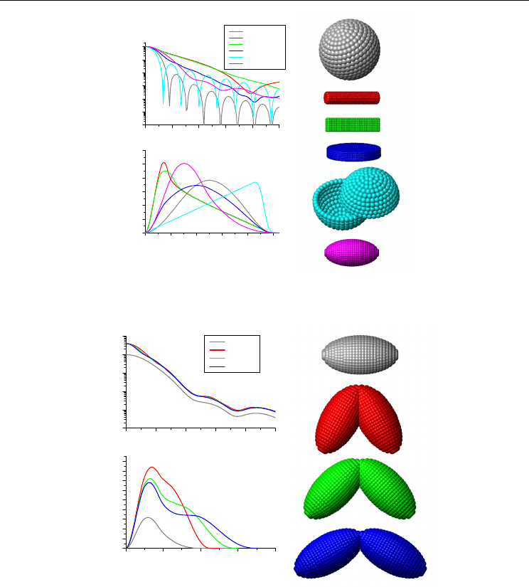
of the particle shape and electron density distribution. A set of theoretical calculations for

the

p(r) function is shown in Fig5, Fig6 and Fig7. In Fig5 one can see that globular particles

Investigating Macromolecular Complexes in Solution by Small Angle X-Ray Scattering

375

0.0 0.2 0.4 0.6 0.8 1.0

0 1020304050

p(r)

r/D

MAX

Intensity

MAX

Solid Sphere

Long Cylinder

Long Prism

Flat Particle

Hollow Sphere

Prolate ellipsoid

Fig. 5. Theoretical calculations for scattering intensities and corresponding

p(r) functions for

bodies with simple shapes. The form factors were normalized to one.

0 20406080

0.0 0.2 0.4 0.6 0.8 1.0

p(r)

r [Å]

Intensity

q [Å

-1

]

Monomer

Dimer 60

Dimer 90

Dimer 120

Fig. 6. Theoretical calculations for scattering intensities and corresponding

p(r) functions for

bodies with simple shapes. The form factors were normalized by the forward scattering of

the monomer.

will have a

p(r) function with a bell shape, with the maximum close to (r/D

MAX

)/2. Any

anisotropy will move the maximum to the left, towards lower

r/D

MAX

values. Elongated

(prolate) particles with constant cross-section like cylinders or prisms will have

p(r)

functions with linearly descent regions. Flat (oblate) particles will have

p(r) functions with

shapes different from the two previous cases. Hollow particles will have

p(r) functions with

the maximum moved to the right, towards higher

r/D

MAX

values. Dimeric particles will have

p(r) with shoulders, as viewed in Fig6. Interestingly, the differences in the opening angle of a

Current Trends in X-Ray Crystallography

376

dimeric particle are easier to detect in the p(r) function than in the intensity I(q). Finally,

particles with differences in the scattering length contrast might have

p(r) functions with

negative portions as indicated in Fig7. For a broader and deeper review on the

p(r)

interpretation the reader is invited to read several works in the literature (Glatter, 1979;

Glatter and Kratky, 1982). The important point of this modeling approach is that, apart from

the assumption that the system is composed of identical particles, no other hypothesis are

made and the

p(r) function provides a direct insight about the particle shape and

dimensions. This approach is widely used in analysis of SAXS data because it provides a

first guess about the particle shape.

0 5 10 15 20 25

I(q)

MAX

Core-Shell particle

0.0 0.2 0.4 0.6 0.8 1.0

p(r)

r/D

MAX

Fig. 7. Theoretical calculations for scattering intensities and corresponding

p(r) functions for

a core-shell particle with different scattering length contrasts.

2.2.2 Model dependent approach – assuming a known form factor

For simple particle shapes it is possible to integrate equation (2) and obtain the amplitude

form factor







. Then, performing the angular integral given in equation (6) it is possible

to obtain a analytical or semi-analytical expression for





. Some examples are shown in

Table 1. A more complete list of analytical expressions for form factors can be found in

Shape Normalized Form Factor

Homogeneus sphere with

radius R

 



3sin cosqR qR qR

Iq fq





















Spherical shell with inner

radius R1 and outer radius



 

11 1 22 2

() , () ,

() ()

VR f qR VR f qR

VR VR



















() 4 /3VR R





Homogeneous cylinder

with radius R and height L



2sinsincos/2

sin

sin cos / 2

JqR qL

Iq d

qR qL



















Ellipsoid of revolution

with semi axes R, R and R

  

,( , , )sinIq fqrR d















1/2

(,,) sin cosrR R

   



Table 1. Few examples of semi-analytical expressions of the scattering intensity calculated

for particles with simple shapes.





>0