Boyer George R. An Economic History of the English Poor Law, 1750-1850
Подождите немного. Документ загружается.

The Poor
Law,
Migration, and Economic Growth 111
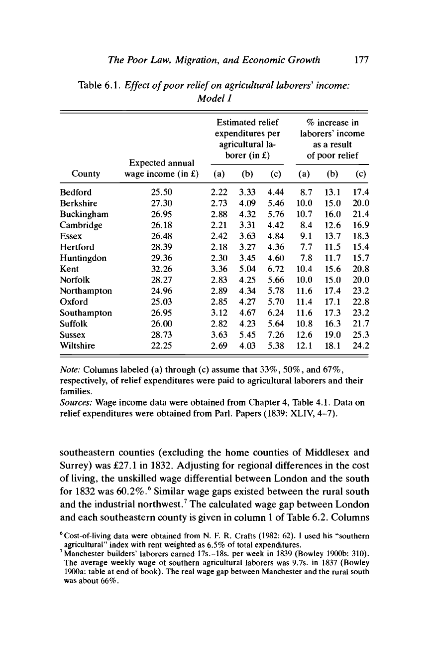
Table 6.1. Effect of poor
relief
on
agricultural
laborers'
income:
Model 1
County
Bedford
Berkshire
Buckingham
Cambridge
Essex
Hertford
Huntingdon
Kent
Norfolk
Northampton
Oxford
Southampton
Suffolk
Sussex
Wiltshire
Exoected annual
wage income
(in £)
25.50
27.30
26.95
26.18
26.48
28.39
29.36
32.26
28.27
24.96
25.03
26.95
26.00
28.73
22.25
Estimated relief
expenditures
per
agriculturalla-
borer (in
£)
(a)
2.22
2.73
2.88
2.21
2.42
2.18
2.30
3.36
2.83
2.89
2.85
3.12
2.82
3.63
2.69
(b)
3.33
4.09
4.32
3.31
3.63
3.27
3.45
5.04
4.25
4.34
4.27
4.67
4.23
5.45
4.03
(c)
4.44
5.46
5.76
4.42
4.84
4.36
4.60
6.72
5.66
5.78
5.70
6.24
5.64
7.26
5.38
%
increasei
in
laborers' income
as
a
result
of
(a)
8.7
10.0
10.7
8.4
9.1
7.7
7.8
10.4
10.0
11.6
11.4
11.6
10.8
12.6
12.1
poor relief
(b)
13.1
15.0
16.0
12.6
13.7
11.5
11.7
15.6
15.0
17.4
17.1
17.3
16.3
19.0
18.1
(c)
17.4
20.0
21.4
16.9
18.3
15.4
15.7
20.8
20.0
23.2
22.8
23.2
21.7
25.3
24.2
Note:
Columns labeled
(a)
through
(c)
assume that
33%,
50%, and 67%,
respectively,
of
relief expenditures were paid
to
agricultural laborers and their
families.
Sources:
Wage income data were obtained from Chapter 4, Table
4.1.
Data
on
relief expenditures were obtained from Parl. Papers (1839: XLIV, 4-7).
southeastern counties (excluding the home counties of Middlesex and
Surrey) was £27.1 in 1832. Adjusting for regional differences in the cost
of living, the unskilled wage differential between London and the south
for 1832 was 60.2%.
6
Similar wage gaps existed between the rural south
and the industrial northwest.
7
The calculated wage gap between London
and each southeastern county is given in column
1
of Table 6.2. Columns
6
Cost-of-living data were obtained from N.
F. R.
Crafts (1982: 62).
I
used
his
"southern
agricultural" index with rent weighted as 6.5%
of
total expenditures.
7
Manchester builders' laborers earned 17s.-18s.
per
week
in
1839 (Bowley 1900b:
310).
The average weekly wage
of
southern agricultural laborers
was
9.7s.
in
1837 (Bowley
1900a: table
at
end
of
book).
The real wage gap between Manchester and the rural south
was about 66%.
178 An Economic History of the English Poor Law
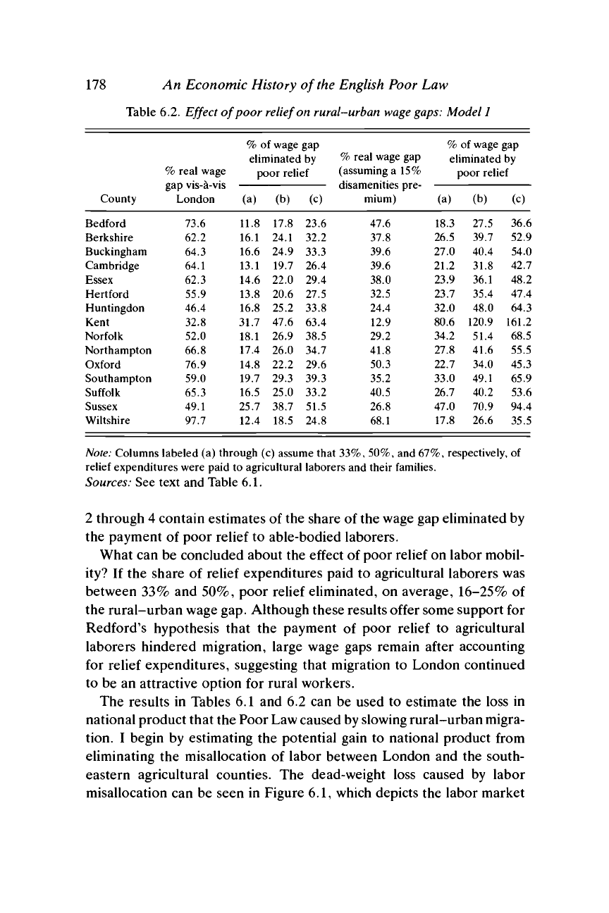
Table 6.2. Effect of poor
relief on
rural-urban
wage
gaps:
Model 1
County
Bedford
Berkshire
Buckingham
Cambridge
Essex
Hertford
Huntingdon
Kent
Norfolk
Northampton
Oxford
Southampton
Suffolk
Sussex
Wiltshire
% real wage
gdp vis-d-vis
London
73.6
62.2
64.3
64.1
62.3
55.9
46.4
32.8
52.0
66.8
76.9
59.0
65.3
49.1
97.7
% of wage
eliminatec
gap
lby
poor relief
(a)
11.8
16.1
16.6
13.1
14.6
13.8
16.8
31.7
18.1
17.4
14.8
19.7
16.5
25.7
12.4
(b)
17.8
24.1
24.9
19.7
22.0
20.6
25.2
47.6
26.9
26.0
22.2
29.3
25.0
38.7
18.5
(c)
23.6
32.2
33.3
26.4
29.4
27.5
33.8
63.4
38.5
34.7
29.6
39.3
33.2
51.5
24.8
% real wage gap
(assuming a 15%
disamenities pre-
mium)
47.6
37.8
39.6
39.6
38.0
32.5
24.4
12.9
29.2
41.8
50.3
35.2
40.5
26.8
68.1
% of wage
gap
eliminated by
(a)
18.3
26.5
27.0
21.2
23.9
23.7
32.0
80.6
34.2
27.8
22.7
33.0
26.7
47.0
17.8
poor relief
(b)
27.5
39.7
40.4
31.8
36.1
35.4
48.0
120.9
51.4
41.6
34.0
49.1
40.2
70.9
26.6
(c)
36.6
52.9
54.0
42.7
48.2
47.4
64.3
161.2
68.5
55.5
45.3
65.9
53.6
94.4
35.5
Note:
Columns labeled (a) through (c) assume that
33%,
50%, and 67%, respectively, of
relief expenditures were paid to agricultural laborers and their families.
Sources:
See text and Table 6.1.
2 through 4 contain estimates of the share of the wage gap eliminated by
the payment of poor relief to able-bodied laborers.
What can be concluded about the effect of poor relief on labor mobil-
ity? If the share of relief expenditures paid to agricultural laborers was
between 33% and 50%, poor relief eliminated, on average, 16-25% of
the rural-urban wage gap. Although these results offer some support for
Redford's hypothesis that the payment of poor relief to agricultural
laborers hindered migration, large wage gaps remain after accounting
for relief expenditures, suggesting that migration to London continued
to be an attractive option for rural workers.
The results in Tables 6.1 and 6.2 can be used to estimate the loss in
national product that the Poor Law caused by slowing rural-urban migra-
tion. I begin by estimating the potential gain to national product from
eliminating the misallocation of labor between London and the south-
eastern agricultural counties. The dead-weight loss caused by labor
misallocation can be seen in Figure 6.1, which depicts the labor market
The Poor
Law,
Migration,
and Economic Growth 179
Marginal Product
and Real Wage in
Manufacturing (m)
Marginal Product
and Real Wage in
Agriculture (a)
I
1
I
1
y
w*
I I*
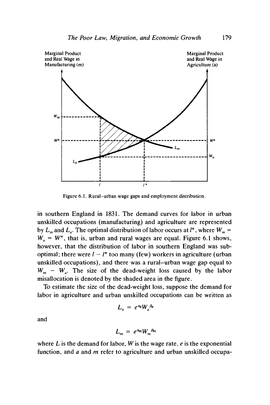
Figure 6.1. Rural-urban wage gaps and employment distribution.
in southern England in 1831. The demand curves for labor in urban
unskilled occupations (manufacturing) and agriculture are represented
by L
m
and L
a
. The optimal distribution of labor occurs at /*, where W
m
=
W
a
= W*, that is, urban and rural wages are equal. Figure 6.1 shows,
however, that the distribution of labor in southern England was sub-
optimal; there were / - /* too many (few) workers in agriculture (urban
unskilled occupations), and there was a rural-urban wage gap equal to
W
m
- W
a
. The size of the dead-weight loss caused by the labor
misallocation is denoted by the shaded area in the figure.
To estimate the size of the dead-weight loss, suppose the demand for
labor in agriculture and urban unskilled occupations can be written as
and
where L is the demand for labor, W
is
the wage rate, e is the exponential
function, and a and m refer to agriculture and urban unskilled occupa-
180 An Economic History of
the
English Poor Law
tions,
respectively. For simplicity, I assume that labor supply equals
labor demand at the existing wage in each sector. Given data on L
fl
, L
m
,
W
a
, and W
m
, and estimates of
/3
a
and /3
m
(the own-wage elasticities of
demand for labor in agriculture and nonagriculture), the equations can
be solved for e
aa
and e
am
. The equilibrium wage rate in the absence of
labor misallocation is then obtained by adding the equations together
and solving for W*. Substituting W* into the original labor demand
equations, one can determine the optimal distribution of labor between
the two sectors, L* and L*. It is then a simple process to determine the
dead-weight social loss caused by the misallocation of labor between
London and the 15 southeastern counties. My choices for
j8
fl
and /3
m
follow Williamson (1987: 659), whose "best guess" estimates of the own-
wage elasticity of demand for labor in agriculture and nonagriculture
were -1.10 and
-0.75,
respectively. Assuming that
j8
fl
= -1.0 and
/3
W
=
-0.75,
the dead-weight loss was equal to £462,000 in 1831, or 0.14% of
national product.
8
While this is a small percentage, it represents 5.6% of
the annual rate of growth of commodity output for 1821 to
1831.
9
How much of the dead-weight loss resulted from the payment of poor
relief to agricultural laborers? If poor relief eliminated 16-25% of the
rural-urban wage gap, one could argue that no more than 25% of the
dead-weight loss can be attributed to the Poor Law. In other words, the
decline in migration caused by poor relief reduced national income by at
most £115,500 in
1831.
10
8
Data
on
national product were obtained from Deane
and
Cole (1967: 166). Williamson
provided
a
range
of
estimates
for the
labor demand elasticities: /3
a
= -0.68 and
-1.10;
/3
m
=
-0.25, -0.75,
and -3.0. I
also estimated
the
loss
in
national product
for
other
values
of the
labor demand elasticities.
For p
a
= -0.5 and fi
m
=
-0.75,
the
estimated
dead-weight loss
was
£335,000.
For p
a
= -0.5 and
/3
W
= -1.0, the
estimated dead-
weight loss was £377,000.
For
(3
a
=
-1.0 and
/3
m
=
-1.0,
the
estimated dead-weight loss
equaled £546,000.
For p
a
= -0.5 and
j8
m
= -1.5, the
estimated dead-weight loss
was
£430,000. Obviously,
the
choice
of
own-wage elasticities does
not
have
a
large effect
on
the estimated loss
in
national product.
9
Commodity output grew
at an
annual rate
of
2.50% from
1821
to
1831 (Crafts
1985:
47).
10
The above calculations assume that
the
rural-urban wage
gap
that remained after poor
relief benefits
are
taken into account reflects
a
disequilibrium
in the
labor market.
A
similar assumption is made by Williamson
(1987:
671-2), who concludes that the English
labor market "failed"
in the
early nineteenth century. Part
of the
wage
gap,
however,
might reflect migration
costs,
rural-urban differences in labor quality, "greater
job
uncer-
tainty
or
the [high] cost
of
job
search" in urban areas,
or
a
compensating
wage
differential
needed
to
attract rural migrants
"to
locations
of
poorer environmental quality" (William-
son
1987:
657,
653).
If
so,
then the above calculations overstate the total dead-weight loss
caused
by
rural-urban
wage gaps
and understate the share of the dead-weight
loss
attribut-
able to the Poor
Law.
The possibility that part of the rural-urban
wage
gap represented an
"urban disamenities premium"
is
addressed later
in
this section.
The Poor
Law,
Migration,
and Economic Growth
181
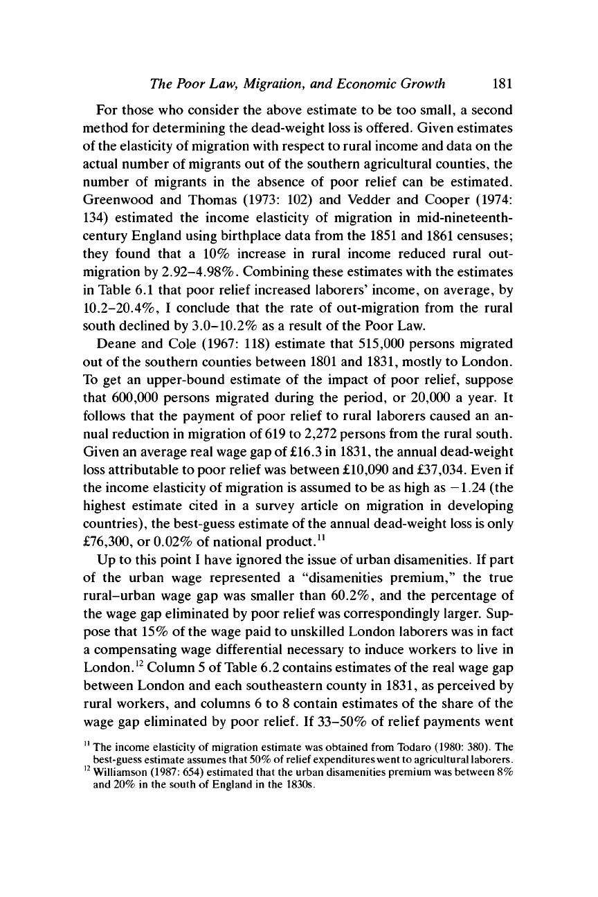
For those
who
consider
the
above estimate
to be too
small,
a
second
method
for
determining
the
dead-weight loss is offered. Given estimates
of the elasticity
of
migration with respect
to
rural income
and
data
on the
actual number
of
migrants
out of the
southern agricultural counties,
the
number
of
migrants
in the
absence
of
poor relief
can be
estimated.
Greenwood
and
Thomas
(1973:
102) and
Vedder
and
Cooper (1974:
134) estimated
the
income elasticity
of
migration
in
mid-nineteenth-
century England using birthplace data from
the
1851
and
1861 censuses;
they found that
a 10%
increase
in
rural income reduced rural
out-
migration
by
2.92-4.98%. Combining these estimates with
the
estimates
in Table
6.1
that poor relief increased laborers' income,
on
average,
by
10.2-20.4%,
I
conclude that
the
rate
of
out-migration from
the
rural
south declined
by
3.0-10.2%
as a
result
of the
Poor
Law.
Deane
and
Cole (1967:
118)
estimate that 515,000 persons migrated
out
of the
southern counties between 1801
and
1831, mostly
to
London.
To
get an
upper-bound estimate
of the
impact
of
poor
relief,
suppose
that 600,000 persons migrated during
the
period,
or
20,000
a
year.
It
follows that
the
payment
of
poor relief
to
rural laborers caused
an an-
nual reduction
in
migration
of
619
to
2,272 persons from
the
rural south.
Given
an
average real wage gap
of
£16.3
in
1831,
the
annual dead-weight
loss attributable
to
poor relief
was
between £10,090
and
£37,034. Even if
the income elasticity
of
migration
is
assumed
to be as
high
as -1.24 (the
highest estimate cited
in a
survey article
on
migration
in
developing
countries),
the
best-guess estimate
of
the annual dead-weight loss is only
£76,300,
or
0.02%
of
national product.
11
Up
to
this point
I
have ignored
the
issue
of
urban disamenities.
If
part
of
the
urban wage represented
a
"disamenities premium,"
the
true
rural-urban wage
gap was
smaller than 60.2%,
and the
percentage
of
the wage
gap
eliminated
by
poor relief was correspondingly larger.
Sup-
pose that 15%
of
the wage paid
to
unskilled London laborers was
in
fact
a compensating wage differential necessary
to
induce workers
to
live
in
London.
12
Column 5
of
Table
6.2
contains estimates
of
the real wage
gap
between London
and
each southeastern county
in
1831,
as
perceived
by
rural workers,
and
columns
6 to 8
contain estimates
of the
share
of the
wage
gap
eliminated
by
poor
relief. If
33-50%
of
relief payments went
11
The
income elasticity
of
migration estimate
was
obtained from Todaro (1980: 380).
The
best-guess estimate assumes that
50%
of
relief expenditures went to agricultural laborers.
12
Williamson (1987: 654) estimated that
the
urban disamenities premium was between
8%
and 20%
in the
south
of
England
in the
1830s.
182 An Economic History of
the
English Poor Law
to agricultural laborers, then the Poor Law eliminated 30-40% of the
wage gap. However, with a 15% disamenities premium the total dead-
weight loss caused by the misallocation of labor in the southeast was
equal to only £182,800 in 1831. If 40% of the dead-weight loss can be
attributed to the payment of poor relief to agricultural laborers, the
decline in national income caused by the Poor Law was about £73,100 in
1831,
or 0.02% of national income.
The above results all lead to the same conclusion. Even if all relief
payments to agricultural laborers were in excess of their marginal prod-
uct, there is no evidence that the Poor Law kept the English economy
from enjoying a large free lunch associated with transferring workers
from low-productivity agricultural jobs to high-productivity urban em-
ployment. Moreover, there are two reasons to believe that the above
results significantly overestimate the effect of poor relief on migration
and national product. First, I have assumed, for simplicity, that relief
expenditures were distributed evenly among agricultural laborers. How-
ever, married men with large families received larger relief payments
than single males or young married men, and young adults dominated
the flow of migrants to English cities.
13
The most mobile group of rural
laborers, therefore, was the group least affected by poor
relief.
Second, the assumption that all relief payments were in excess of
laborers' marginal product is almost certainly incorrect. Labor-hiring
farmers dominated parish politics. They would not have adopted a sys-
tem of poor relief that increased their expenditures per worker above
the marginal product of labor. The second and third models assume that
wage income and poor relief were substitutes. Farmers used the system
of outdoor relief to reduce wage rates below the marginal product of
labor. Rather than increase farmers' labor costs, the Poor Law either
had no effect on farmers' costs or reduced them.
2.
The
Effect
of
Poor Relief
on
Migration:
The
Polanyi Model
The second model assumes that the total compensation package paid by
farmers to their employees (consisting of wages and farmers' contribu-
tion to relief benefits) was equal to labor's marginal product; that is
W + eB = MP
e
13
Williamson (1988: 304-5) estimated that 53.3%
of
the migrants into British cities
in the
1840s were aged 15-29, while only 7.4% were aged 30
or
older.
The Poor
Law,
Migration,
and Economic Growth 183
In other words, the system of outdoor relief enabled farmers to reduce
their wage payments by an amount eB, equal to their contribution to the
poor rate. Farmers' total expenditure on labor was not affected by the
Poor Law, and the difference between laborers' income and their mar-
ginal product was determined solely by the contribution of non-labor-
hiring taxpayers to the poor rate. A laborer's annual income is thus
W + B = MP
e
+ (1 - e)B
where
(1
- e)B
is
the relief payment per worker made
by
non-labor-hiring
taxpayers. The percentage increase in workers' income above the mar-
ginal product of labor brought about by the Poor Law is given by
(1 - e)BIMP
e
= {\- e)B/(W + eB)
Notice that this is precisely the solution to the problem of rising urban
wage rates suggested by Polanyi; farmers used the Poor Law to raise their
laborers' annual incomes without increasing their own payments to labor.
The effect of such a policy on rural-urban migration depends on the
value of (1 - e), the share of poor relief expenditures paid by local
taxpayers other than labor-hiring farmers. I assume that non-labor-
hiring taxpayers and landlords paid
20-33%
of the poor rate in the
typical agricultural parish.
14
Tables 6.3 and 6.4 contain estimates of the
percentage increase in agricultural laborers' annual incomes caused by
the Poor Law, and the percentage of the rural-urban wage gap elimi-
nated by relief payments, for the same counties as before.
15
Table 6.3
assumes that taxpayers who did not hire labor paid 20% of the poor rate,
while Table 6.4 assumes that non-labor-hiring taxpayers paid
33%
of the
poor rate.
The conclusion to be reached from the results is clear. Farmers may
have attempted to use the Poor Law as a dam to "prevent the draining
off of rural labor," as Polanyi contended, but such a policy could not
14
These represent lower- and upper-bound estimates for the value of (1 - e), obtained
from Section 3 of Chapter 3.
15
The differences in the size of rural-urban wage gaps between Tables 6.2, 6.3, and 6.4
follow from my assumption that the proper measure of the rural wage to be used in
calculating wage gaps is the marginal product of labor in agriculture, because that is the
wage that would have existed in the absence of poor
relief.
Table 6.2 assumes that the
marginal product of labor was equal to the observed
wage.
Tables 6.3 and 6.4 assume that
the marginal product of labor equaled W + eB, the observed wage plus the farmer's
contribution to the worker's relief benefit. Thus, the marginal product of labor
is
larger in
Tables 6.3 and 6.4 than in Table 6.2, and therefore the estimated rural-urban wage gaps
are smaller
in
Tables 6.3 and 6.4 than
in
Table
6.2.
The
wage gaps
differ between Tables 6.3
and 6.4 because I assume that e = 0.80 in Table 6.3 and that e = 0.67 in Table 6.4.
184
An
Economic History of the
English
Poor
Law
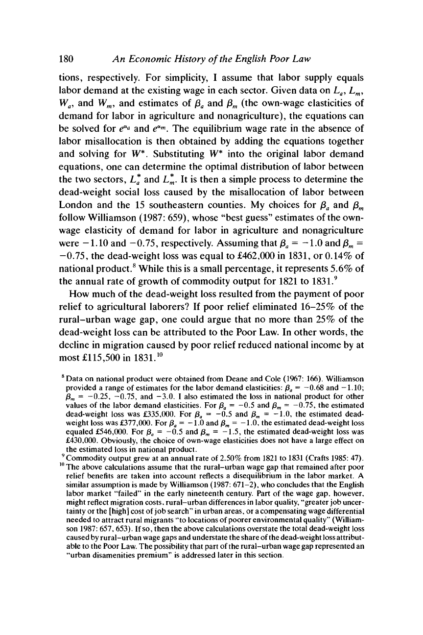
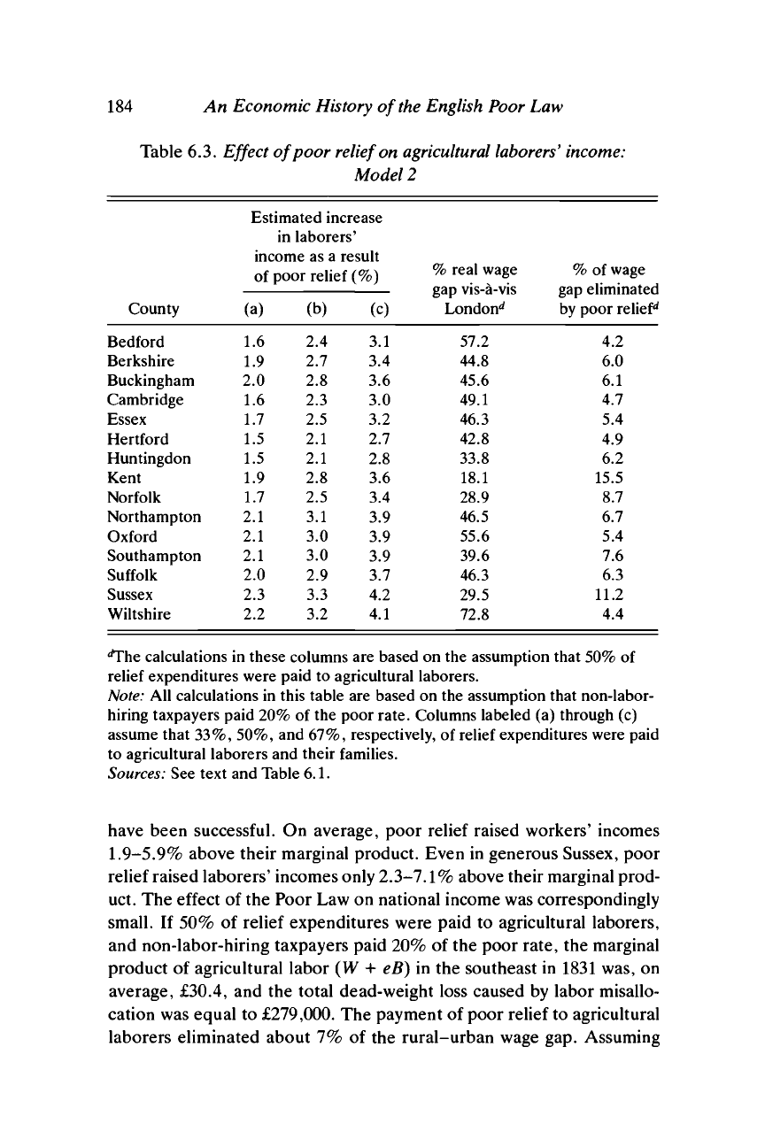
Table 6.3. Effect of poor relief on
agricultural
laborers'
income:
Model
2
County
Bedford
Berkshire
Buckingham
Cambridge
Essex
Hertford
Huntingdon
Kent
Norfolk
Northampton
Oxford
Southampton
Suffolk
Sussex
Wiltshire
Estimated increase
in laborer!
income
of poor
(a)
1.6
1.9
2.0
1.6
1.7
1.5
1.5
1.9
1.7
2.1
2.1
2.1
2.0
2.3
2.2
as a result
relief (%)
(b)
2.4
2.7
2.8
2.3
2.5
2.1
2.1
2.8
2.5
3.1
3.0
3.0
2.9
3.3
3.2
(c)
3.1
3.4
3.6
3.0
3.2
2.7
2.8
3.6
3.4
3.9
3.9
3.9
3.7
4.2
4.1
%
real wage
gap vis-a-vis
London**
57.2
44.8
45.6
49.1
46.3
42.8
33.8
18.1
28.9
46.5
55.6
39.6
46.3
29.5
72.8
%
of wage
gap eliminated
by poor
relief*
4.2
6.0
6.1
4.7
5.4
4.9
6.2
15.5
8.7
6.7
5.4
7.6
6.3
11.2
4.4
calculations in these columns are based on the assumption that 50% of
relief expenditures were paid to agricultural laborers.
Note: All calculations in this table are based on the assumption that non-labor-
hiring taxpayers paid 20% of the poor rate. Columns labeled (a) through (c)
assume that 33%, 50%, and 67%, respectively, of relief expenditures were paid
to agricultural laborers and their families.
Sources: See text and Table 6.1.
have been successful.
On
average, poor relief raised workers' incomes
1.9-5.9%
above their marginal product. Even
in
generous Sussex, poor
relief raised laborers' incomes only
2.3-7.1%
above their marginal prod-
uct.
The
effect
of
the Poor Law
on
national income was correspondingly
small.
If
50%
of
relief expenditures were paid
to
agricultural laborers,
and non-labor-hiring taxpayers paid 20%
of
the poor rate,
the
marginal
product
of
agricultural labor
(W + eB) in the
southeast
in
1831
was, on
average, £30.4,
and the
total dead-weight loss caused
by
labor misallo-
cation was equal
to
£279,000.
The
payment
of
poor relief to agricultural
laborers eliminated about
7% of the
rural-urban wage
gap.
Assuming

The
Poor
Law,
Migration,
and Economic Growth
185
Table
6.4. Effect
of poor relief on agricultural
laborers'
income:
Model
2
County
Bedford
Berkshire
Buckingham
Cambridge
Essex
Hertford
Huntingdon
Kent
Norfolk
Northampton
Oxford
Southampton
Suffolk
Sussex
Wiltshire
Estimated increase
in laborer*
income as a result
of poor relief (%)
(a)
2.7
3.1
3.3
2.6
2.8
2.4
2.5
3.2
3.1
3.5
3.5
3.5
3.3
3.8
3.7
(b)
4.0
4.5
4.8
3.8
4.1
3.5
3.6
4.7
4.5
5.1
5.1
5.1
4.8
5.6
5.3
(c)
5.1
5.8
6.2
5.0
5.4
4.6
4.7
6.0
5.8
6.6
6.5
6.6
6.3
7.1
6.9
% real wage
gar) vis-a-vis
London**
59.6
47.4
48.4
51.4
48.7
44.8
35.7
20.2
38.1
49.5
58.7
42.5
49.1
32.3
76.4
% of wage
t?ao eliminated
gUL/
VlltlllIli4VVVt
by poor
relief^
6.7
9.5
9.9
7.4
8.4
7.8
10.1
23.3
11.8
10.3
8.7
12.0
9.8
17.3
6.9
calculations in these columns are based on the assumption that 50% of
relief expenditures were paid to agricultural laborers.
Note:
All calculations in this table are based on the assumption that non-labor-
hiring taxpayers paid
33%
of the poor rate. Columns labeled (a) through (c)
assume that
33%,
50%, and 67%, respectively, of relief expenditures were paid
to agricultural laborers and their families.
Sources:
See text and Table 6.1.
that
7% of the dead-weight loss is attributable to poor
relief,
the decline
in
national income caused by the Poor Law
was
about
£19,500
in
1831.
If
non-labor-hiring
taxpayers paid
33%
of the poor rate, the dead-weight
loss
attributable to the Poor Law was about £33,400 in 1831.
The
impact of the Poor Law was even smaller if part of the London
wage
represented an urban disamenities premium. Columns 1 and 2 of
Table
6.5 contain estimates of the wage gap between London and each
southeastern
county, as perceived by rural workers, assuming a 15%
disamenities
premium, and columns 3 and 4 contain estimates of the
share
of the wage gap eliminated by poor
relief.
If
50%
of relief expen-
186 An Economic History of
the
English Poor Law
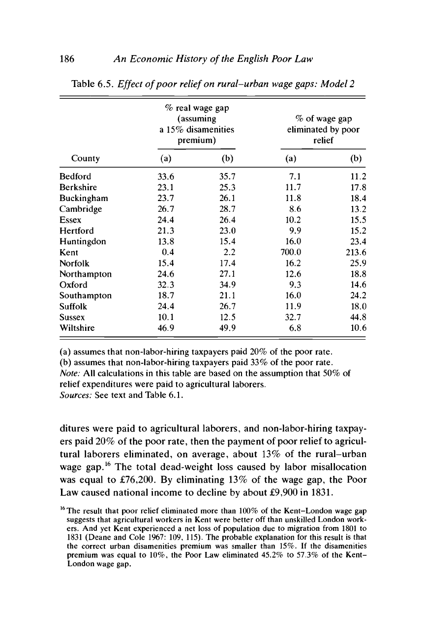
Table 6.5. Effect of poor relief on rural-urban
wage
gaps:
Model 2
County
Bedford
Berkshire
Buckingham
Cambridge
Essex
Hertford
Huntingdon
Kent
Norfolk
Northampton
Oxford
Southampton
Suffolk
Sussex
Wiltshire
% real wage
gap
(assuming
a 15% disamenities
(a)
33.6
23.1
23.7
26.7
24.4
21.3
13.8
0.4
15.4
24.6
32.3
18.7
24.4
10.1
46.9
premium)
(b)
35.7
25.3
26.1
28.7
26.4
23.0
15.4
2.2
17.4
27.1
34.9
21.1
26.7
12.5
49.9
%
of wage
gap
eliminated
by
poor
(a)
7.1
11.7
11.8
8.6
10.2
9.9
16.0
700.0
16.2
12.6
9.3
16.0
11.9
32.7
6.8
relief
(b)
11.2
17.8
18.4
13.2
15.5
15.2
23.4
213.6
25.9
18.8
14.6
24.2
18.0
44.8
10.6
(a) assumes that non-labor-hiring taxpayers paid 20%
of
the poor rate.
(b) assumes that non-labor-hiring taxpayers paid
33%
of
the poor rate.
Note:
All
calculations
in
this table
are
based
on the
assumption that 50%
of
relief expenditures were paid
to
agricultural laborers.
Sources:
See
text
and
Table 6.1.
ditures were paid to agricultural laborers, and non-labor-hiring taxpay-
ers paid 20% of the poor rate, then the payment of poor relief to agricul-
tural laborers eliminated, on average, about 13% of the rural-urban
wage gap.
16
The total dead-weight loss caused by labor misallocation
was equal to £76,200. By eliminating 13% of the wage gap, the Poor
Law caused national income to decline by about £9,900 in 1831.
16
The result that poor relief eliminated more than 100%
of the
Kent-London wage
gap
suggests that agricultural workers
in
Kent were better
off
than unskilled London work-
ers.
And yet
Kent experienced
a net
loss
of
population
due to
migration from 1801
to
1831 (Deane
and
Cole 1967:
109,
115).
The
probable explanation
for
this result
is
that
the correct urban disamenities premium
was
smaller than
15%. If the
disamenities
premium
was
equal
to 10%, the
Poor
Law
eliminated 45.2%
to
57.3%
of the
Kent-
London wage
gap.