Baumgarte T., Shapiro S. Numerical Relativity. Solving Einstein’s Equations on the Computer
Подождите немного. Документ загружается.


Appendix F Collisionless matter evolution in axisymmetry 631
An attractive feature of this equation for the lapse is that the simple flat space form of the 3-
dimensional Laplacian appears on the left hand side. Imposing the quasi-isotropic spatial gauge
conditions (F. 2 ) leads to a system of coupled first-order equations for the two shift components,
8
β
r
and β
θ
:
r∂
r
β
r
r
− ∂
θ
β
θ
=
α
A
2
B
(2
ˆ
λ − 3
ˆ
K
φ
φ
), (F.12)
r∂
r
β
θ
+ ∂
θ
β
r
r
=
2α
A
2
Br
ˆ
K
r
θ
. (F.13)
In spherical symmetry, the above equations reduce to those presented in Chapter 8.2.The
variable η is a measure of the deviation from spherical symmetry since η = 0 in spherical
spacetimes. In an asymptotically flat, axisymmetric spacetime, η also measures the even-parity
gravitational wave amplitude at large distances according to
η = h
TT
+
+ O(r
−2
). (F.14)
According to equation (F. 5 ), we also have ∂
t
η → λ as r →∞. With h
TT
×
= 0 in the absence of
rotation, we can then use equation (9.30) to compute the energy loss due to gravitational radiation,
dE
dt
=−
1
16π
lim
r→∞
r
2
dλ
2
. (F.15)
No angular momentum is carried off by gravitational waves in axisymmetry.
Matter equations
The geodesic equations of motion for the collisionless particles are:
dr
dt
=
αu
r
A
2
− β
r
, (F.16)
dθ
dt
=
αu
θ
A
2
r
2
− β
θ
, (F.17)
dφ
dt
=
α
B
2
r
2
sin
2
θ
u
φ
, (F.18)
du
r
dt
=−∂
r
α + u
r
∂
r
β
r
+ u
θ
∂
r
β
θ
−
α
2
∂
r
1
A
2
u
2
r
+ ∂
r
1
r
2
A
2
u
2
θ
+ ∂
r
1
B
2
r
2
u
2
φ
sin
2
θ
, (F.19)
du
θ
dt
=−∂
θ
α + u
r
∂
θ
β
r
+ u
θ
∂
θ
β
θ
−
α
2
&
∂
θ
1
A
2
u
2
r
+ ∂
θ
1
r
2
A
2
u
2
θ
+ ∂
θ
1
B
2
r
2
sin
2
θ
u
2
φ
'
, (F.20)
du
φ
dt
= 0, (F.21)
8
See Evans (1984), p. 121, for a proof that this is an elliptic system.

632 Appendix F Collisionless matter evolution in axisymmetry
where the normalization condition u
µ
u
µ
=−1gives
≡ αu
0
=
1 +
u
2
r
A
2
+
u
2
θ
r
2
A
2
+
u
2
φ
B
2
r
2
sin
2
θ
1/2
. (F.22)
Assuming that all N particles have the same rest mass m = M
0
/N , where M
0
is the total rest
mass of the system, they may be binned to determine the source terms for the field equations as
follows:
ˆρ =
j
m
j
(r
2
sin θrθ φ)
j
, (F.23)
ˆ
S
r
=
j
mu
j
r
(r
2
sin θrθ φ)
j
, (F.24)
ˆ
S
θ
=
j
mu
j
θ
(r
2
sin θrθ φ)
j
, (F.25)
ˆ
S
rθ
=
j
mu
j
r
u
j
θ
j
(r
2
sin θrθ φ)
j
, (F.26)
ˆ
S = ˆρ −
j
m
j
(r
2
sin θrθ φ)
j
. (F.27)
Since the particles are distributed axisymmetrically in rings the bin width φ can be set to 2π.
Disks
The above scheme is easily adapted to treat infinitely thin, axisymmetric disks of matter residing
in the equatorial plane.
9
In this case, “jump” conditions satisfied by the field variables across the
equator replace the usual matter source terms that appear in the field equations. As an example of
how the jump conditions are obtained, consider equation (F. 9 ). Functions like
ˆ
K
r
r
,
ˆ
K
φ
φ
and η are
symmetric across the equatorial plane and continuous there. Multiplying the equation by rsinθ
and integrating across the equator therefore yields
0 =
+
−
ˆ
S
r
rsinθdθ −
1
r
ˆ
K
r
θ
|
+
−
, (F.28)
where ± denotes θ = π/2 ± , → 0. Since
ˆ
K
r
θ
is antisymmetric across the equator, equa-
tion (F. 2 8 )gives
ˆ
K
r
θ
|
+
=−
ˆ
K
r
θ
|
−
=
r
2
+
−
ˆ
S
r
rsinθdθ. (F.29)
The jump condition (F. 2 9 ) is used to set the value of
ˆ
K
r
θ
at the boundary of an integration along
the equatorial plane. In the vacuum outside of the equatorial plane,
ˆ
K
r
θ
is determined by evolving
equation (F. 6 ) in the usual way. Since particles are confined to the equatorial plane where β
θ
= 0,
9
Abrahams et al. (1994, 1995).

Appendix F Collisionless matter evolution in axisymmetry 633
the particle 4-velocity satisfies u
θ
= u
θ
= 0, hence S
θ
= 0. Integrating equation (F. 8 ) across the
equator then reduces to 0 = 0.
In a similar fashion, integration of the Hamiltonian constraint equation (F. 1 0 )gives
1
r
sinθ∂
θ
ψ|
+
=−
1
4r
ψ∂
θ
η|
+
−
1
8ψ
+
−
ˆρr sinθdθ. (F.30)
Integrating the lapse equation (F. 1 1 ) yields
1
r
sinθ∂
θ
(αψ)|
+
=−
1
4r
αψ∂
θ
η|
+
+
1
8
αψ
B
+
−
(ˆρ + 2
ˆ
S)r sinθ dθ. (F.31)
In finite differencing, say, the Hamiltonian constraint, the derivative terms ∂
θ
ψ and ∂
θ
η appear
in exactly the same combination as in the jump condition (F. 3 0 ). Thus the only place where the
matter source term appears is through the boundary conditions. The same result holds for the
lapse equation.
The evolution equation (F. 5 )forη and the shift equations (F. 1 2 ) and (F. 1 3 )forβ
r
and β
φ
do
not contain any matter sources and remain unchanged. We recall that η, β
r
and β
φ
are metric
coefficients and must be continuous across the equator.
The geodesic equations for the particles are unchanged, except for the simplification that
θ = π/2 and u
θ
= 0. Accordingly, only the radial motion of the particles is dynamical in an
infinitely thin, axisymmetric disk, as in spherical symmetry.
The matter source terms appearing in the jump conditions can be determined by binning the
particles in radial annuli, yielding
ˆσ ≡
+
−
ˆρr sinθdθ =
j
m
j
(2πr r)
j
, (F.32)
ˆ
r
≡
+
−
ˆ
S
r
r sinθ dθ =
j
m(u
r
)
j
(2πr r)
j
, (F.33)
ˆ
≡
+
−
ˆ
Sr sinθdθ = ˆσ −
j
m
j
(2πr r)
j
. (F.34)
Once again, the particle rest mass m is related to the total rest mass M
0
by m = M
0
/N , where N
is the total particle number. The rest mass can be found from
M
0
=
ˆσ
0
2πrdr, (F.35)
where
ˆσ
0
≡
+
−
ˆρ
r sinθ dθ =
j
m
(2πr r)
j
. (F.36)
G
Rotating equilibria:
gravitational field equations
In this appendix we assemble the gravitational field equations that are required to construct numer-
ical models of rotating, relativistic, equilibrium configurations, such as the rotating fluid stars
discussed in Chapter 14 and the rotating collisionless clusters discussed in Chapters 10 and 14.
Following Komatsu et al. (1989a) we assume stationary equilibrium and write the spacetime
metric in the form (14.1),
ds
2
=−e
γ +ρ
dt
2
+ e
2σ
(dr
2
+r
2
dθ
2
) + e
γ −ρ
r
2
sin
2
θ(dφ − ωdt)
2
, (G.1)
where the metric potentials ρ, γ , ω, and σ are functions of r and θ only. Einstein’s equations G
ab
=
8π T
ab
then provide three elliptic equations (14.2)–(14.4) for the metric potentials ρ, γ and ω,
∇
2
[ρe
γ/2
] = S
ρ
(r,µ), (G.2)
∇
2
+
1
r
∂
r
−
µ
r
2
∂
µ
[γ e
γ/2
] = S
γ
(r,µ), (G.3)
∇
2
+
2
r
∂
r
−
2µ
r
2
∂
µ
[ωe
(γ −2ρ)/2
] = S
ω
(r,µ), (G.4)
where ∇
2
is the flat-space Laplace operator in spherical polar coordinates and µ = cos θ.The
effective sources terms S
ρ
, S
γ
and S
ω
are given by
S
ρ
(r,µ) = e
γ/2
1
r
∂
r
γ −
µ
r
2
∂
µ
γ +
ρ
2
&
−∂
r
γ
1
2
∂
r
γ +
1
r
−
1
r
2
∂
µ
γ
1 − µ
2
2
∂
µ
γ − µ
'
+r
2
(1 − µ
2
)e
−2ρ
(∂
r
ω)
2
+
1 − µ
2
r
2
(∂
µ
ω)
2
+8π e
2σ
T
ˆ
φ
ˆ
φ
− T
ˆ
t
ˆ
t
+
ρ
2
(T
ˆ
r
ˆ
r
+ T
ˆ
θ
ˆ
θ
)
(G.5)
S
γ
(r,µ) = e
γ/2
γ
2
&
−
1
2
(∂
r
γ )
2
−
1 − µ
2
2r
2
(∂
µ
γ )
2
'
+ 8π e
2σ
1 +
γ
2
(T
ˆ
r
ˆ
r
+ T
ˆ
θ
ˆ
θ
)
-
, (G.6)
S
ω
(r,µ) = e
(γ −2ρ)/2
ω
&
−
1
r
2∂
r
ρ +
1
2
∂
r
γ
+
µ
r
2
2∂
µ
ρ +
1
2
∂
µ
γ
+
1
4
4(∂
r
ρ)
2
− (∂
r
γ )
2
+
1 − µ
2
4r
2
4(∂
µ
ρ)
2
− (∂
µ
γ )
2
−r
2
(1 − µ
2
)e
−2ρ
(∂
r
ω)
2
+
1 − µ
2
r
2
(∂
µ
ω)
2
'
+8π e
2σ
−ω(T
ˆ
φ
ˆ
φ
− T
ˆ
t
ˆ
t
) +
ω
2
(T
ˆ
r
ˆ
r
+ T
ˆ
θ
ˆ
θ
) −
2e
ρ
T
ˆ
t
ˆ
φ
r(1 − µ
2
)
1/2
. (G.7)
634

Appendix G Rotating equilibria 635
Here T
ˆ
a
ˆ
b
are the orthonormal components of the stress-energy tensor for matter as observed
by a normal observer, n
a
. In the literature dealing with stationary, rotating equilibria, normal
observers are often referred to as zero angular momentum observers (ZAMOs).
1
We purposely
leave the stress-energy tensor unspecified to allow for different matter models
2
(see Chapter 5
for some astrophysically relevant examples).
The fourth field equation determines σ and is given by
∂
µ
σ =−
1
2
(∂
µ
ρ + ∂
µ
γ ) −{(1 − µ
2
)(1 + r∂
r
γ )
2
+ [µ − (1 − µ
2
)∂
µ
γ ]
2
}
−1
×
1
2
[r
2
(∂
2
r
γ + (∂
r
γ )
2
) − (1 − µ
2
)(∂
2
µ
γ + (∂
µ
γ )
2
)][−µ + (1 − µ
2
)∂
µ
γ ]
+r∂
r
γ
&
1
2
µ + µr∂
r
γ +
1
2
(1 − µ
2
)∂
µ
γ
'
+
3
2
∂
µ
γ [−µ
2
+ µ(1 − µ
2
)∂
µ
γ ]
−r(1 −µ
2
)
∂
r
∂
µ
γ + (∂
r
γ )(∂
µ
γ )
(1 + r∂
r
γ ) −
1
4
µr
2
(∂
r
ρ + ∂
r
γ )
2
−
r
2
(1 − µ
2
)(∂
r
ρ + ∂
r
γ )(∂
µ
ρ + ∂
µ
γ ) +
1
4
µ(1 − µ
2
)(∂
µ
ρ + ∂
µ
γ )
2
−
r
2
2
(1 − µ
2
)∂
r
γ (∂
r
ρ + ∂
r
γ )(∂
µ
ρ + ∂
µ
γ )
+
1
4
(1 − µ
2
)∂
µ
γ [r
2
(∂
r
ρ + ∂
r
γ )
2
− (1 − µ
2
)(∂
µ
ρ + ∂
µ
γ )
2
]
+(1 − µ
2
)e
−2ρ
&
1
4
r
4
µ(∂
r
ω)
2
+
1
2
r
3
(1 − µ
2
)(∂
r
ω)(∂
µ
ω) −
1
4
r
2
µ(1 − µ
2
)(∂
µ
ω)
2
+
1
2
r
4
(1 − µ
2
)(∂
r
γ )(∂
r
ω)(∂
µ
ω) −
1
4
r
2
(1 − µ
2
)∂
µ
γ [r
2
(∂
r
ω)
2
− (1 − µ
2
)(∂
µ
ω)
2
]
'
−r
2
[µ − (1 − µ
2
)∂
µ
γ ]e
2σ
4π(T
ˆ
r
ˆ
r
− T
ˆ
θ
ˆ
θ
) + r
2
(1 − µ
2
)
1/2
(1 + r∂
r
γ )e
2σ
8π T
ˆ
r
ˆ
θ
.
(G.8)
The equations for the metric components assembled by Komatsu et al. (1989a) and listed above
are most easily derived by projecting the Einstein field equations onto the orthonormal tetrad of
aZAMO.
Following Komatsu et al. (1989a), the integral Green function solutions to the three elliptical
field equations (G.2)–(G.4)are
ρ =−e
−γ/2
∞
n=0
∞
0
dr
1
0
dµ
r
2
f
2
2n
(r, r
)P
2n
(µ)P
2n
(µ
)S
ρ
(r
,µ
), (G.9)
γ =−
2
π
e
−γ/2
r sin θ
∞
n=1
∞
0
dr
1
0
dµ
r
2
f
1
2n−1
(r, r
)
2n − 1
sin
(
(2n − 1)θ
)
sin
(2n − 1)θ
S
γ
(r
,µ
),
(G.10)
1
Bardeen (1973).
2
Shapiro and Teukolsky (1993a).

636 Appendix G Rotating equilibria
ω =−
e
(2ρ−γ )/2
r sin θ
∞
n=1
∞
0
dr
1
0
dµ
r
3
sin θ
f
2
2n−1
(r, r
)
2n(2n − 1)
P
1
2n−1
(µ)P
1
2n−1
(µ
)S
ω
(r
,µ
),
(G.11)
where
f
1
n
(r, r
) =
(r
/r)
n
, for r
/r ≤ 1,
(r/r
)
n
, for r
/r > 1,
(G.12)
and
f
2
n
(r, r
) =
(1/r)(r
/r)
n
, for r
/r ≤ 1,
(1/r
)(r/r
)
n
, for r
/r > 1.
(G.13)
Here the P
n
are Legendre polynomials and the P
m
n
are associated Legendre functions. Equa-
tion (G.8)forσ is solved by integrating the linear ordinary differential equation from the pole
(µ = 1) to the equator with the initial condition that
σ =
γ − ρ
2
at µ = 1, (G.14)
which arises from the requirement of local flatness on the coordinate axis.
The coupled equations for the gravitational and matter fields can be solved by a stable iteration
scheme like the one described in Komatsu et al. (1989a) for fluid stars.
3
It is modeled after the
approach devised by Hachisu (1986) for Newtonian systems. The integral equations can be solved
on a discrete 2-dimensional spatial grid covering the computational domain over a large but finite
radius, 0 ≤ r ≤ r
max
and 0 ≤ µ ≤ 1. In the implementation by Cook et al. (1992), a coordinate
transformation to a new radial coordinate s, defined by
r = r
e
s
1 − s
, 0 ≤ s ≤ 1, (G.15)
allows us to extend the computational domain to spatial infinity (r
max
=∞). Here r
e
is the radius
of the surface of the matter at the equator. Derivatives of quantities appearing in the effective
source terms are handled by finite differencing.
3
See Chapter 14.1.2 for a brief sketch.

H
Moving puncture
representions of
Schwarzschild:
analytical results
As we discussed in Chapter 13.1.3, moving puncture simulations typically employ the 1+log
slicing condition (4.51),
∂
t
α − β
i
∂
i
α =−2αK. (H.1)
We also pointed out that moving puncture simulations that start with Schwarzschild initial data
– specifically, the v = 0 time slice of Schwarzschild in a Kruskal–Szekeres diagram (Figure 1.1)
– settle down asymptotically to a stationary solution. In this appendix we derive some analytical
representations of these asymptotic solutions. These solutions are very valuable for two reasons:
they provide very useful code tests,
1
and help delineate the geometrical properties of moving
puncture solutions.
Maximal slicing
Let us first consider a “nonadvective” version of the 1+log slicing condition (H.1), i.e.,
∂
t
α =−2αK. (H.2)
If at late times the solution settles down and becomes time-independent, we must have ∂
t
α = 0,
implying that the late-time solution must be maximally sliced with K = 0. The solution must
therefore be a member of the family of time-independent, maximal slicings of Schwarzschild
described by equations (4.23)–(4.25) and parametrized by the constant C. Hannam et al. (2007)
show that evolving with the Gamma-driver shift condition (4.83) yields the late-time solution
corresponding to the particular member C = 3
√
3M
2
/4, which has a limiting surface at the areal
radius r
s
= 3M/2. The family (4.23)–(4.25) is expressed in terms of an areal radius r
s
,butfor
numerical purposes it is often more convenient to express this solution in terms of an isotropic
radius r. As it turns out, the cases C = 0 (see exercise 3.4) and C = 3
√
3M
2
/4aretheonly
cases for which these solutions can be expressed in isotropic coordinates in terms of elementary
functions.
2
Exercise H.1 (a) To transform from the areal radius r
s
in (4.23) to an isotropic
radius r, identify the spatial metric (4.23) with its counterpart in isotropic, polar
1
Employing moving puncture gauge conditions, and using these solutions as initial data, should result in a time-
independent solution. Any nonzero time evolution is therefore a measure of the numerical error.
2
The remainder of this section follows Baumgarte and Naculich (2007).
637

638 Appendix H Moving puncture representions of Schwarzschild
coordinates, γ
ij
= ψ
4
η
ij
. Show that this yields
ψ =
r
s
r
1/2
(H.3)
as well as the differential equation
±
dr
r
=
r
s
dr
s
r
4
s
− 2Mr
3
s
+ C
2
. (H.4)
(b) In the general case the right-hand side of equation (H.4) may be expressed in
terms of elliptic integrals. The integral simplifies, however, for C = 0 (in which
case we recover the situation of exercise 3.4), and for C = 3
√
3M
2
/4. Show that
for C = 3
√
3M
2
/4 the quartic polynomial in equation (H.4) has a double root at
r
s
= 3M/2, and show that integration yields
r =
2r
s
+ M + (4r
2
s
+ 4Mr
s
+ 3M
2
)
1/2
4
×
(4 + 3
√
2)(2r
s
− 3M)
8r
s
+ 6M + 3(8r
2
s
+ 8Mr
s
+ 6M
2
)
1/2
1/
√
2
, (H.5)
where a constant of integration has been fixed so that r → r
s
as r
s
→∞. Also show
that r → 0asr
s
→ 3M/2.
Given equation (H.5) we can now construct the entire spacetime metric
ds
2
=−α
2
dt
2
+ ψ
4
η
ij
(dx
i
+ β
i
dt)(dx
j
+ β
j
dt)(H.6)
as follows. From equation (H.3) we find the conformal factor
ψ =
4r
s
2r
s
+ M + (4r
2
s
+ 4Mr
s
+ 3M
2
)
1/2
1/2
8r
s
+ 6M + 3(8r
2
s
+ 8Mr
s
+ 6M
2
)
1/2
(4 + 3
√
2)(2r
s
− 3M)
1/2
√
2
.
(H.7)
To express ψ in terms of the isotropic radius r would require inverting equation (H.5); clearly that
is not possible. Instead, equations (H.5) and (H.7) together provide a parametric representation of
ψ(r). Exercise H.2 demonstrates that the conformal factor features a 1/
√
r coordinate singularity
at r = 0, so that this point corresponds to a surface of finite areal radius r
s
(cf. exercise 13.1). We
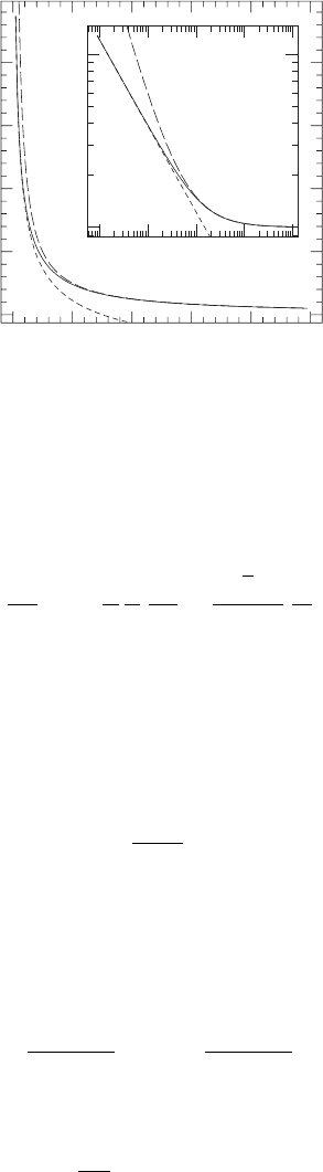
show ψ(r) together with its asymptotic limits in Figure H.1.
Exercise H.2 Show that the conformal factor (H.7) has the expected asymptotic
limits
ψ →
3M
2r
1/2
r → 0
1 +
M
2r
r →∞.
(H.8)
The lapse α in equation (4.24) transforms like a scalar under spatial coordinate transformations
and hence remains
α =
1 −
2M
r
s
+
27M
4
16r
4
s
1/2
, (H.9)
Appendix H Moving puncture representions of Schwarzschild 639
0
5
10
4
3
34 5
100
10
0.1
0.01
2
2
r/M
1
1
y
1
1
Figure H.1 The conformal factor ψ (equation H.7) for the maximally sliced asymptotic solution (solid lines),
together with its asymptotic limits (equation H.8) (dashed lines), as functions of the isotropic radius r.[From
Baumgarte and Naculich (2007).]
while the shift has to be transformed from the areal radius r
s
in equation (4.25) to the isotropic
radius r,
β
r
=
dr
dr
s
β
r
s
=
r
r
s
1
f
Cf
r
2
s
=
3
√
3M
2
4
r
r
3
s
. (H.10)
Both the lapse and shift can again be represented parametrically in terms of r.
Stationary 1+log slicing
Now let us return to the “advective” 1+log slicing condition (H.1). The time-independent, asymp-
totic solution must then satisfy
3
K =
β
i
∂
i
α
2α
. (H.11)
We can construct these slices using the same “height-function” approach that we used in Chapter
4.2 to find the family of maximal slices (4.23)–(4.25). Recall that, starting with the standard
Schwarzschild coordinates, we introduced a new time coordinate
¯
t = t + h(r
s
), where t is the
original Schwarzschild time and h(r
s
) the height function. We then identified the lapse and the
shift on
¯
t = constant surfaces and found the expressions (4.18)
β
r
s
=
f
2
0
h
1 − f
2
0
h
2
,α
2
=
f
0
1 − f
2
0
h
2
, (H.12)
where h
≡ dh/dr
s
and f
0
(r
s
) = 1 − 2M/r
s
. It is now convenient to express h
in terms of the
lapse,
h
=
1
α f
0
α
2
− f
0
1/2
, (H.13)
3
This section follows Hannam et al. (2008).
640 Appendix H Moving puncture representions of Schwarzschild
so that the shift becomes
β
r
s
= α
α
2
− f
0
1/2
. (H.14)
From equation (4.19) we can also show that
K =
1
r
2
s
d
dr
s
r
2
s
f
0
αh
=
1
r
2
s
d
dr
s
r
2
s
α
2
− f
0
1/2
. (H.15)
Inserting the shift (H.14) and the mean curvature (H.15) into the slicing condition (H.11) then
yields a differential equation for the lapse
dα
dr
s
=−
2
r
s
3M − 2r
s
+ 2r
s
α
2
r
s
− 2M + 2r
s
α − r
s
α
2
. (H.16)
Exercise H.3 Show that the differential equation (H.16) is solved by the implicit
equation
α
2
= 1 −
2M
r
s
+
C
2
e
α
r
4
s
(H.17)
for any value of the constant C.
Remarkably, the solution (H.17) for the lapse differs from the maximal slicing result (4.24)
only by the exponential term e
α
. This term complicates matters considerably, of course, since now
the lapse is given only implicitly. As for the maximal slicing case, again we have discovered an
entire family of solutions that satisfies the slicing condition (H.11), and again we can parametrize
this family in terms of the constant C.
We notice, however, that the solutions may become singular if the denominator in equation
(H.16) vanishes. To ensure that the solution remains regular we demand that the numerator of the
equation vanish simultaneously with the denominator; this condition determines the constant C.
The numerator of equation (H.16) vanishes when
α =
1 −
3M
2r
s
1/2
(H.18)
(where we have chosen the positive root). Given this value of the lapse, the denominator of
equation (H.16) vanishes at a critical radius r
c
given by
r
c
=
3 +
√
10
4
M. (H.19)
At r
c
, the lapse is
α
c
=
√
10 − 3. (H.20)
We can now insert both equations (H.19) and (H.20) into equation (H.17), which yields
C =
√
2
16
(
√
10 + 3)
3/2
e
(3−
√
10)/2
M
2
1.24672M
2
. (H.21)
This value of C identifies the member of the family in which we are interested. Substituting C into
equation (H.17) we can then find, at least implicitly, α for all values of the areal radius r
s
. Knowing
α we can find h
from equation (H.13), which then determines all other metric quantities.
Exercise H.4 (a) Recall that the 1+log slicing condition (H.1) is a member of a
larger family of slicing conditions (4.49)
∂
t
α − β
i
∂
i
α =−α
2
f (α)K (H.22)