Banner A. The Calculus Lifesaver: All the Tools You Need to Excel at Calculus
Подождите немного. Документ загружается.


696 • Limits and Proofs
differentiate g and see what that means for f. Since the quantities f(b) −f(a)
and b − a are constant, we get
g
0
(x) = f
0
(x) −
f(b) − f(a)
b − a
.
Now plug in x = c. Since g
0
(c) = 0, we have
0 = f
0
(c) −
f(b) − f(a)
b − a
.
This means that
f
0
(c) =
f(b) − f(a)
b − a
,
which is exactly what we wanted to show!
A.6.9 The error in linearization
Let’s tie up another loose end. In Section 13.2 of Chapter 13, we looked at
the linearization L of a function f about x = a, where a is some number in
the domain of f:
L(x) = f(a) + f
0
(a)(x − a).
If x is near a, we can use L(x) to estimate the value of f (x). How wrong could
we possibly be? According to the formula in Section 13.2.4 of Chapter 13, if
f
00
exists between x and a, then
|error| =
1
2
|f
00
(c)||x − a|
2
;
here c is some number between x and a. Let’s prove this formula. Start off by
calling the error term r(x); since r(x) is the difference between the true value
f(x) and our guess, which is the linearization L(x) = f(a) + f
0
(a)(x − a), we
have
r(x) = f (x) − L(x) = f(x) − f (a) − f
0
(a)(x − a).
Now, the clever idea is to fix x as a constant and let a be the variable. Inspired
by this, let
g(t) = f(x) − f (t) − f
0
(t)(x − t).
So the error r(x) arises exactly when t = a. That is, the error is g(a). Note
that
g(x) = f(x) − f (x) − f
0
(x)(x − x) = 0.
Let’s differentiate g with respect to t. The term f(x) is constant, so its
derivative is 0. Also, we need the product rule to deal with f
0
(t)(x − t). All
in all, we get
g
0
(t) = 0 − f
0
(t) − (f
0
(t) × (−1) + f
00
(t)(x − t)) = −f
00
(t)(x − t).
In particular, we have
g
0
(x) = −f
00
(x)(x − x) = 0.

Section A.6.10: Derivatives of piecewise-defined functions • 697
Everything we’ve done so far makes a lot of sense. Now we have to do some-
thing that seems to be a little whacked out. Remember that we want to show
that the error is
1
2
f
00
(c)(x − a)
2
, where c is between x and a. Since the error
is g(a), this suggests that g(t) is something like K(x − t)
2
, where K is some
number which does not depend on t, but only on x and a. Even this isn’t
exactly true, but it might explain why we’re going to let
h(t) = g(t) − K(x − t)
2
.
You see, when you differentiate this with respect to t, holding x constant, you
get
h
0
(t) = g
0
(t) + 2K(x − t).
So what? Well, we can use the Mean Value Theorem (see Section 11.3 of
Chapter 11) to get
h
0
(c) =
h(x) − h(a)
x − a
for some c between x and a. We can substitute for h
0
(c), h(x), and h(a) using
the above equations:
g
0
(c) + 2K(x − c) =
(g(x) − K(x − x)
2
) − (g(a) − K(x − a)
2
)
x − a
=
−g(a) + K(x − a)
2
x − a
,
since g(x) = 0. Since g
0
(c) = −f
00
(c)(x − c), this last equation can be rear-
ranged to
g(a) − K(x − a)
2
= (x − a)(x − c)(f
00
(c) − 2K).
We’re close, but there’s still a problem. We can’t handle the factor (x − c),
since that’s nowhere to be found in our error term! The only way we can get
rid of it is if the left-hand side is actually 0. That is, we should have chosen
K such that g(a) − K(x − a)
2
= 0. Indeed, if K = g(a)/(x − a)
2
, then the
above equation becomes
0 = (x − a)(x − c)
f
00
(c) −
2g(a)
(x − a)
2
.
Since x 6= a and x 6= c, we must have
f
00
(c) −
2g(a)
(x − a)
2
= 0,
which means that g(a) =
1
2
f
00
(c)(x −a)
2
. Since g(a) = r(x) is the error we’re
looking for, we’re finished.
A.6.10 Derivatives of piecewise-defined functions
Imagine that f is defined in piecewise fashion as
f(x) =
(
f
1
(x) if x > a,
f
2
(x) if x ≤ a.

698 • Limits and Proofs
(You could change x > a to x ≥ a, and x ≤ a to x < a; it doesn’t make a
difference.) Anyway, in Section 6.6 of Chapter 6, we considered the question
of whether f is differentiable at a. We have assumed that if the functions f
1
and f
2
match at x = a, and also the derivatives f
0
1
and f
0
2
match at x = a,
then f is differentiable at a. How can we justify this? Well, first note that
the matching of f
1
and f
2
at x = a means that
lim
x→a
+
f
1
(x) = lim
x→a
−
f
2
(x) = f(a).
This ensures that f is at least continuous. Now we are also assuming that the
derivatives match: this means that f
1
is differentiable to the immediate right
of a, f
2
is differentiable to the immediate left of a, and
lim
x→a
+
f
0
1
(x) = lim
x→a
−
f
0
2
(x) = L,
where L is some nice finite number. So consider the quantity
f(a + h) − f(a)
h
for some small number h 6= 0. If h > 0, then we can apply the Mean Value
Theorem (see Section 11.3 of Chapter 11) to say that
f(a + h) − f(a)
h
= f
0
1
(c),
where c is some number between a and a + h. (Here we needed the continuity
of f on [a, a + h].) By the sandwich principle, as h → 0
+
, the number c is
sandwiched between a and a + h, so c → a
+
as h → 0
+
. We now see that
lim
h→0
+
f(a + h) − f(a)
h
= lim
h→0
+
f
0
1
(c) = lim
c→a
+
f
0
1
(c) = L.
The left-hand limit works the same way, except that we use f
0
2
instead of f
0
1
to see that
lim
h→0
−
f(a + h) − f (a)
h
= lim
h→0
−
f
0
2
(c) = lim
c→a
−
f
0
2
(c) = L.
The left-hand and right-hand limits are both equal to L, so we have shown
that f
0
(a) exists and is also equal to L.
A.6.11 Proof of l’Hopital’s Rule
b
Let’s prove l’Hˆopital’s Rule (see Chapter 14). Specifically, suppose we
have two functions f and g which are both differentiable on some interval
containing a point a (but maybe not at a itself); and f(a) = g(a) = 0; and
also g
0
(x) 6= 0 except maybe at a itself. Then we need to show that
lim
x→a
f(x)
g(x)
= lim
x→a
f
0
(x)
g
0
(x)
,
provided that the limit on the right-hand side exists. We’ll need a slightly
different version of the Mean Value Theorem, called Cauchy’s Mean Value

Section A.6.11: Proof of l’Hˆopital’s Rule • 699
Theorem: if f and g are continuous on [A, B] and differentiable on (A, B),
and also g
0
(x) 6= 0 on (A, B), then there is some C in (A, B) such that
f
0
(C)
g
0
(C)
=
f(B) − f(A)
g(B) − g(A)
.
Let’s prove this first, then use it to prove l’Hˆopital’s Rule. Incidentally, note
that if g(x) = x for all x, then g
0
(x) = 1 and the above equation becomes
f
0
(C) =
f(B) − f(A)
B − A
.
This is just the regular Mean Value Theorem! That doesn’t really help us,
though. Let’s go back to the original equation above and look at the denom-
inator on the right-hand side, which is g(B) − g(A). That can’t be equal to
0; if it were, then g(A) = g(B), meaning that g
0
(C) = 0 for some C in (A, B)
by Rolle’s Theorem (see Section 11 in Chapter 11.2). So the right-hand side
makes sense. Now, define a new function h by
h(x) = f(x) −
f(B) − f(A)
g(B) − g(A)
g(x)
for all x in (A, B). (Compare this with the function we called g in the proof
of the ordinary Mean Value Theorem in Section A.6.8 above.) Anyway, let’s
write down some nice facts about this function. First, let’s calculate h(A) and
h(B). We have
h(A) = f(A) −
f(B) − f(A)
g(B) − g(A)
g(A)
=
f(A)g(B) − f(A)g(A) − f (B)g(A) + f(A)g(A)
g(B) − g(A)
=
f(A)g(B) − f(B)g(A)
g(B) − g(A)
,
whereas
h(B) = f(B) −
f(B) − f(A)
g(B) − g(A)
g(B)
=
f(B)g(B) − f(B)g(A) − f(B)g(B) + f (A)g(B)
g(B) − g(A)
=
f(A)g(B) − f(B)g(A)
g(B) − g(A)
.
So h(A) = h(B). Also, note that h is differentiable, and since A and B are
constant, we have
h
0
(x) = f
0
(x) −
f(B) − f(A)
g(B) − g(A)
g
0
(x).
We can use Rolle’s Theorem, since h(A) = h(B), to conclude that there’s a
number C in (A, B) such that h
0
(C) = 0. This means that
h
0
(C) = f
0
(C) −
f(B) − f(A)
g(B) − g(A)
g
0
(C) = 0.
700 • Limits and Proofs
If you rearrange this equation, you get the one we want:
f
0
(C)
g
0
(C)
=
f(B) − f(A)
g(B) − g(A)
.
Now we’re ready to prove l’Hˆopital’s Rule. Since f(a) = g(a) = 0, we have
lim
x→a
f(x)
g(x)
= lim
x→a
f(x) − f (a)
g(x) − g(a)
.
If x > a, then we can use Cauchy’s Mean Value Theorem (which we just
proved) on the interval [a, x] to say that
lim
x→a
f(x)
g(x)
= lim
x→a
f(x) − f (a)
g(x) − g(a)
= lim
x→a
f
0
(c)
g
0
(c)
for some c in (a, x). Otherwise, if x < a, then the same thing is true but c
is in (x, a). (Note that we’ve used the fact that g
0
isn’t 0, except possibly at
a; that’s one of the conditions of Cauchy’s Mean Value Theorem.) Of course,
the number c depends on what x is; but we can see that as x → a, also c → a.
So we have
lim
x→a
f(x)
g(x)
= lim
x→a
f
0
(c)
g
0
(c)
= lim
c→a
f
0
(c)
g
0
(c)
.
All that’s left is to treat c as the dummy variable and change it to x, and
l’Hˆopital’s Rule is proved!
Well, sort of. We still haven’t proved the ∞/∞ case, nor the case when
x → ∞ (or −∞). It’s a great exercise to try to adapt the above proof to these
PSfrag
replacements
(
a, b)
[
a, b]
(
a, b]
[
a, b)
(
a, ∞)
[
a, ∞)
(
−∞, b)
(
−∞, b]
(
−∞, ∞)
{
x : a < x < b}
{
x : a ≤ x ≤ b}
{
x : a < x ≤ b}
{
x : a ≤ x < b}
{
x : x ≥ a}
{
x : x > a}
{
x : x ≤ b}
{
x : x < b}
R
a
b
shado
w
0
1
4
−
2
3
−
3
g(
x) = x
2
f(
x) = x
3
g(
x) = x
2
f(
x) = x
3
mirror
(y = x)
f
−
1
(x) =
3
√
x
y = h
(x)
y = h
−
1
(x)
y =
(x − 1)
2
−
1
x
Same
height
−
x
Same
length,
opp
osite signs
y = −
2x
−
2
1
y =
1
2
x − 1
2
−
1
y =
2
x
y =
10
x
y =
2
−x
y =
log
2
(x)
4
3
units
mirror
(x-axis)
y = |
x|
y = |
log
2
(x)|
θ radians
θ units
30
◦
=
π
6
45
◦
=
π
4
60
◦
=
π
3
120
◦
=
2
π
3
135
◦
=
3
π
4
150
◦
=
5
π
6
90
◦
=
π
2
180
◦
= π
210
◦
=
7
π
6
225
◦
=
5
π
4
240
◦
=
4
π
3
270
◦
=
3
π
2
300
◦
=
5
π
3
315
◦
=
7
π
4
330
◦
=
11
π
6
0
◦
=
0 radians
θ
hyp
otenuse
opp
osite
adjacen
t
0
(≡ 2π)
π
2
π
3
π
2
I
I
I
I
II
IV
θ
(
x, y)
x
y
r
7
π
6
reference
angle
reference
angle =
π
6
sin
+
sin −
cos
+
cos −
tan
+
tan −
A
S
T
C
7
π
4
9
π
13
5
π
6
(this
angle is
5π
6
clo
ckwise)
1
2
1
2
3
4
5
6
0
−
1
−
2
−
3
−
4
−
5
−
6
−
3π
−
5
π
2
−
2π
−
3
π
2
−
π
−
π
2
3
π
3
π
5
π
2
2
π
3
π
2
π
π
2
y =
sin(x)
1
0
−
1
−
3π
−
5
π
2
−
2π
−
3
π
2
−
π
−
π
2
3
π
5
π
2
2
π
2
π
3
π
2
π
π
2
y =
sin(x)
y =
cos(x)
−
π
2
π
2
y =
tan(x), −
π
2
<
x <
π
2
0
−
π
2
π
2
y =
tan(x)
−
2π
−
3π
−
5
π
2
−
3
π
2
−
π
−
π
2
π
2
3
π
3
π
5
π
2
2
π
3
π
2
π
y =
sec(x)
y =
csc(x)
y =
cot(x)
y = f(
x)
−
1
1
2
y = g(
x)
3
y = h
(x)
4
5
−
2
f(
x) =
1
x
g(
x) =
1
x
2
etc.
0
1
π
1
2
π
1
3
π
1
4
π
1
5
π
1
6
π
1
7
π
g(
x) = sin
1
x
1
0
−
1
L
10
100
200
y =
π
2
y = −
π
2
y =
tan
−1
(x)
π
2
π
y =
sin(
x)
x
,
x > 3
0
1
−
1
a
L
f(
x) = x sin (1/x)
(0 <
x < 0.3)
h
(x) = x
g(
x) = −x
a
L
lim
x
→a
+
f(x) = L
lim
x
→a
+
f(x) = ∞
lim
x
→a
+
f(x) = −∞
lim
x
→a
+
f(x) DNE
lim
x
→a
−
f(x) = L
lim
x
→a
−
f(x) = ∞
lim
x
→a
−
f(x) = −∞
lim
x
→a
−
f(x) DNE
M
}
lim
x
→a
−
f(x) = M
lim
x
→a
f(x) = L
lim
x
→a
f(x) DNE
lim
x
→∞
f(x) = L
lim
x
→∞
f(x) = ∞
lim
x
→∞
f(x) = −∞
lim
x
→∞
f(x) DNE
lim
x
→−∞
f(x) = L
lim
x
→−∞
f(x) = ∞
lim
x
→−∞
f(x) = −∞
lim
x
→−∞
f(x) DNE
lim
x →a
+
f(
x) = ∞
lim
x →a
+
f(
x) = −∞
lim
x →a
−
f(
x) = ∞
lim
x →a
−
f(
x) = −∞
lim
x →a
f(
x) = ∞
lim
x →a
f(
x) = −∞
lim
x →a
f(
x) DNE
y = f (
x)
a
y =
|
x|
x
1
−
1
y =
|
x + 2|
x +
2
1
−
1
−
2
1
2
3
4
a
a
b
y = x sin
1
x
y = x
y = −
x
a
b
c
d
C
a
b
c
d
−
1
0
1
2
3
time
y
t
u
(
t, f(t))
(
u, f(u))
time
y
t
u
y
x
(
x, f(x))
y = |
x|
(
z, f(z))
z
y = f(
x)
a
tangen
t at x = a
b
tangen
t at x = b
c
tangen
t at x = c
y = x
2
tangen
t
at x = −
1
u
v
uv
u +
∆u
v +
∆v
(
u + ∆u)(v + ∆v)
∆
u
∆
v
u
∆v
v∆
u
∆
u∆v
y = f(
x)
1
2
−
2
y = |
x
2
− 4|
y = x
2
− 4
y = −
2x + 5
y = g(
x)
1
2
3
4
5
6
7
8
9
0
−
1
−
2
−
3
−
4
−
5
−
6
y = f (
x)
3
−
3
3
−
3
0
−
1
2
easy
hard
flat
y = f
0
(
x)
3
−
3
0
−
1
2
1
−
1
y =
sin(x)
y = x
x
A
B
O
1
C
D
sin(
x)
tan(
x)
y =
sin(
x)
x
π
2
π
1
−
1
x =
0
a =
0
x
> 0
a
> 0
x
< 0
a
< 0
rest
position
+
−
y = x
2
sin
1
x
N
A
B
H
a
b
c
O
H
A
B
C
D
h
r
R
θ
1000
2000
α
β
p
h
y = g(
x) = log
b
(x)
y = f(
x) = b
x
y = e
x
5
10
1
2
3
4
0
−
1
−
2
−
3
−
4
y =
ln(x)
y =
cosh(x)
y =
sinh(x)
y =
tanh(x)
y =
sech(x)
y =
csch(x)
y =
coth(x)
1
−
1
y = f(
x)
original
function
in
verse function
slop
e = 0 at (x, y)
slop
e is infinite at (y, x)
−
108
2
5
1
2
1
2
3
4
5
6
0
−
1
−
2
−
3
−
4
−
5
−
6
−
3π
−
5
π
2
−
2π
−
3
π
2
−
π
−
π
2
3
π
3
π
5
π
2
2
π
3
π
2
π
π
2
y =
sin(x)
1
0
−
1
−
3π
−
5
π
2
−
2π
−
3
π
2
−
π
−
π
2
3
π
5
π
2
2
π
2
π
3
π
2
π
π
2
y =
sin(x)
y =
sin(x), −
π
2
≤ x ≤
π
2
−
2
−
1
0
2
π
2
−
π
2
y =
sin
−1
(x)
y =
cos(x)
π
π
2
y =
cos
−1
(x)
−
π
2
1
x
α
β
y =
tan(x)
y =
tan(x)
1
y =
tan
−1
(x)
y =
sec(x)
y =
sec
−1
(x)
y =
csc
−1
(x)
y =
cot
−1
(x)
1
y =
cosh
−1
(x)
y =
sinh
−1
(x)
y =
tanh
−1
(x)
y =
sech
−1
(x)
y =
csch
−1
(x)
y =
coth
−1
(x)
(0
, 3)
(2
, −1)
(5
, 2)
(7
, 0)
(
−1, 44)
(0
, 1)
(1
, −12)
(2
, 305)
y =
1
2
(2
, 3)
y = f(
x)
y = g(
x)
a
b
c
a
b
c
s
c
0
c
1
(
a, f(a))
(
b, f(b))
1
2
1
2
3
4
5
6
0
−
1
−
2
−
3
−
4
−
5
−
6
−
3π
−
5
π
2
−
2π
−
3
π
2
−
π
−
π
2
3
π
3
π
5
π
2
2
π
3
π
2
π
π
2
y =
sin(x)
1
0
−
1
−
3π
−
5
π
2
−
2π
−
3
π
2
−
π
−
π
2
3
π
5
π
2
2
π
2
π
3
π
2
π
π
2
c
OR
Lo
cal maximum
Lo
cal minimum
Horizon
tal point of inflection
1
e
y = f
0
(
x)
y = f (
x) = x ln(x)
−
1
e
?
y = f(
x) = x
3
y = g(
x) = x
4
x
f(
x)
−
3
−
2
−
1
0
1
2
1
2
3
4
+
−
?
1
5
6
3
f
0
(
x)
2 −
1
2
√
6
2
+
1
2
√
6
f
00
(
x)
7
8
g
00
(
x)
f
00
(
x)
0
y =
(
x − 3)(x − 1)
2
x
3
(
x + 2)
y = x ln
(x)
1
e
−
1
e
5
−
108
2
α
β
2 −
1
2
√
6
2
+
1
2
√
6
y = x
2
(
x − 5)
3
−
e
−
1/2
√
3
e
−
1/2
√
3
−
e
−3/2
e
−
3/2
−
1
√
3
1
√
3
−
1
1
y = xe
−
3x
2
/2
y =
x
3
− 6
x
2
+ 13x − 8
x
28
2
600
500
400
300
200
100
0
−
100
−
200
−
300
−
400
−
500
−
600
0
10
−
10
5
−
5
20
−
20
15
−
15
0
4
5
6
x
P
0
(
x)
+
−
−
existing
fence
new
fence
enclosure
A
h
b
H
99
100
101
h
dA/dh
r
h
1
2
7
shallo
w
deep
LAND
SEA
N
y
z
s
t
3
11
9
L
(11)
√
11
y = L
(x)
y = f (
x)
11
y = L
(x)
y = f(
x)
F
P
a
a +
∆x
f(
a + ∆x)
L
(a + ∆x)
f(
a)
error
d
f
∆
x
a
b
y = f(
x)
true
zero
starting
approximation
b
etter approximation
v
t
3
5
50
40
60
4
20
30
25
t
1
t
2
t
3
t
4
t
n
−2
t
n
−1
t
0
= a
t
n
= b
v
1
v
2
v
3
v
4
v
n
−1
v
n
−
30
6
30
|
v|
a
b
p
q
c
v(
c)
v(
c
1
)
v(
c
2
)
v(
c
3
)
v(
c
4
)
v(
c
5
)
v(
c
6
)
t
1
t
2
t
3
t
4
t
5
c
1
c
2
c
3
c
4
c
5
c
6
t
0
=
a
t
6
=
b
t
16
=
b
t
10
=
b
a
b
x
y
y = f(
x)
1
2
y = x
5
0
−
2
y =
1
a
b
y =
sin(x)
π
−
π
0
−
1
−
2
0
2
4
y = x
2
0
1
2
3
4
2
n
4
n
6
n
2(
n−2)
n
2(
n−1)
n
2
n
n
=
2
width
of each interval =
2
n
−
2
1
3
0
I
I
I
I
II
IV
4
y
dx
y = −
x
2
− 2x + 3
3
−
5
y = |−
x
2
− 2x + 3|
I
I
I
I
Ia
5
3
0
1
2
a
b
y = f (
x)
y = g(
x)
y = x
2
a
b
5
3
0
1
2
y =
√
x
2
√
2
2
2
dy
x
2
a
b
y = f(
x)
y = g(
x)
M
m
1
2
−
1
−
2
0
y = e
−
x
2
1
2
e
−
1/4
f
a
v
y = f
a
v
c
A
M
0
1
2
a
b
x
t
y = f (
t)
F (
x )
y = f (
t)
F (
x + h)
x + h
F (
x + h) − F (x)
f(
x)
1
2
y =
sin(x)
π
−
π
−
1
−
2
y =
1
x
y = x
2
1
2
1
−
1
y =
ln|x|
θ
a
x
a
x
p
a
2
− x
2
3
x
p
9 − x
2
p
x
2
+ a
2
x
a
p
x
2
+ 15
x
√
15
x
p
x
2
− a
2
a
x
p
x
2
− 4
2
x
−
p
x
2
− a
2
a
x
−
p
x
2
− 4
2
y = f(
x)
a
b
a + ε
ε
Z
b
a
+ε
f(x) dx
small
ev
en smaller
y = g(
x)
infinite
area
finite
area
1
y =
1
x
y =
1
x
p
, p
< 1 (typical)
y =
1
x
p
, p
> 1 (typical)
a
1
a
2
a
3
a
4
a
5
a
6
a
7
a
8
1
2
3
4
5
6
7
8
n
a
n
x
y
y = f(
x)
(
a, f(a))
a
−
1
0
1
a
6
1
2
7
1
2
7
?
−
2
−
1
−
2
t =
0
t = π
/6
t = π
/4
t = π
/3
t = π
/2
3
0
t = −
2
t = −
3/2
t = ±
1
t = −
1/2
t =
0
t =
1/2
t =
3/2
t =
2
12
−
12
θ
r
P
θ
r
P
11
π
6
2
(
−1, −1)
wrong
point
π
4
5
π
4
√
2
(0
, 1)
(0
, −3)
(
−2, 0)
π
2
3
π
2
π
r =
3 sin(θ)
3
π
2
θ
2
π
1
0
−
1
−
2
−
3
0
3
2
−
3
2
0
r =
1 + 2 cos(θ)
2
π
3
4
π
3
0
π
0
pi
−
3
2
3
π
2
1
2
3
0
−
1
−
2
−
3
0 ≤ θ ≤
2
π
3
0 ≤ θ ≤ π
0 ≤ θ ≤ 2
π
r =
1 + cos(θ)
r =
1 +
3
4
cos(
θ)
−
1
4
r =
sin(2θ)
r =
sin(3θ)
r =
1
π
θ
0 ≤ θ ≤ 4
π
r =
2
1
+ sin(θ)
−
π
4
≤ θ ≤
5
π
4
0 ≤ θ ≤ 2
π
0 ≤ θ ≤ π
−
4
−
5
4
5
f(
θ)
f(
θ + dθ)
θ
dθ
θ + dθ
appro
ximating region
exact
region
0 ≤ θ ≤ 2
π
r = |
1 + 2 cos(θ)|
2
i
2 − 3
i
−
1
θ =
0
θ =
π
4
θ =
π
2
θ =
2π
3
θ = π
θ =
13π
12
θ =
3π
2
θ =
7π
4
1 = e
0
e
i
π
4
i = e
i
π
2
e
i
2π
3
−1 = e
iπ
e
i
13π
12
−i = e
i
3π
2
e
i
7π
4
i
−i
1
θ
1 − i
2i
−2i
2
−2
6i
−6i
6
−6
−
√
3
R
ϕ
2
1/5
θ =
π
6
θ =
17π
30
θ =
29π
30
θ =
41π
30
θ =
53π
30
z
0
z
1
z
2
z
3
z
4
−
√
3
2
√
3
2
1
2
i
−i
19π
6
−i
7π
6
i
5π
6
i
17π
6
i
29π
6
ln(2)
−
7π
4
−
3π
4
π
4
5π
4
9π
4
3
2
i
0
1
2
3
4
dx
y
x
y =
p
1 − (x − 3)
2
2πx
a
b
y = f(x)
A
B
y =
√
x
1
y = 2x
3
y = x
4
(2, 16)
−5
5
6
y = h
y−h
h−y
x = h
y
x−h
radius of shell = x−h
h−x
radius of shell = h−x
8
P
h
P
(slice)
(axis)
l
L
1
2
Base
Cross-section
Area = A
Area = A(x)
y = e
x
A
B
dx
dy
x + dx
a
b
p
(dx)
2
+ (dy)
2
P
t
600000
500000
400000
300000
200000
100000
−100000
−200000
−300000
−400000
−500000
−600000
0
1
2
3
4
5
6
7
L
ε
L + ε
L − ε
a
M
a + δ
a − δ
your move
my move
N
M
a + δ
a − δ
your move
my move
FIRST MOVE
SECOND MOVE
L + ε
L − ε
1
−1
L −
1
2
L +
1
2
L = 0
L = −
1
4
L =
7
8
L = 0
b
each segment is either the right half
or the left half of the one below it
infinitely many marked points
lie below each segment
cases, if you dare.
A.7 Proof of the Taylor Approximation Theorem
Now let’s look at how to prove the Taylor approximation theorem from Sec-
PSfrag
replacements
(
a, b)
[
a, b]
(
a, b]
[
a, b)
(
a, ∞)
[
a, ∞)
(
−∞, b)
(
−∞, b]
(
−∞, ∞)
{
x : a < x < b}
{
x : a ≤ x ≤ b}
{
x : a < x ≤ b}
{
x : a ≤ x < b}
{
x : x ≥ a}
{
x : x > a}
{
x : x ≤ b}
{
x : x < b}
R
a
b
shado
w
0
1
4
−
2
3
−
3
g(
x) = x
2
f(
x) = x
3
g(
x) = x
2
f(
x) = x
3
mirror
(y = x)
f
−
1
(x) =
3
√
x
y = h
(x)
y = h
−
1
(x)
y =
(x − 1)
2
−
1
x
Same
height
−
x
Same
length,
opp
osite signs
y = −
2x
−
2
1
y =
1
2
x − 1
2
−
1
y =
2
x
y =
10
x
y =
2
−x
y =
log
2
(x)
4
3
units
mirror
(x-axis)
y = |
x|
y = |
log
2
(x)|
θ radians
θ units
30
◦
=
π
6
45
◦
=
π
4
60
◦
=
π
3
120
◦
=
2
π
3
135
◦
=
3
π
4
150
◦
=
5
π
6
90
◦
=
π
2
180
◦
= π
210
◦
=
7
π
6
225
◦
=
5
π
4
240
◦
=
4
π
3
270
◦
=
3
π
2
300
◦
=
5
π
3
315
◦
=
7
π
4
330
◦
=
11
π
6
0
◦
=
0 radians
θ
hyp
otenuse
opp
osite
adjacen
t
0
(≡ 2π)
π
2
π
3
π
2
I
I
I
I
II
IV
θ
(
x, y)
x
y
r
7
π
6
reference
angle
reference
angle =
π
6
sin
+
sin −
cos
+
cos −
tan
+
tan −
A
S
T
C
7
π
4
9
π
13
5
π
6
(this
angle is
5π
6
clo
ckwise)
1
2
1
2
3
4
5
6
0
−
1
−
2
−
3
−
4
−
5
−
6
−
3π
−
5
π
2
−
2π
−
3
π
2
−
π
−
π
2
3
π
3
π
5
π
2
2
π
3
π
2
π
π
2
y =
sin(x)
1
0
−
1
−
3π
−
5
π
2
−
2π
−
3
π
2
−
π
−
π
2
3
π
5
π
2
2
π
2
π
3
π
2
π
π
2
y =
sin(x)
y =
cos(x)
−
π
2
π
2
y =
tan(x), −
π
2
<
x <
π
2
0
−
π
2
π
2
y =
tan(x)
−
2π
−
3π
−
5
π
2
−
3
π
2
−
π
−
π
2
π
2
3
π
3
π
5
π
2
2
π
3
π
2
π
y =
sec(x)
y =
csc(x)
y =
cot(x)
y = f(
x)
−
1
1
2
y = g(
x)
3
y = h
(x)
4
5
−
2
f(
x) =
1
x
g(
x) =
1
x
2
etc.
0
1
π
1
2
π
1
3
π
1
4
π
1
5
π
1
6
π
1
7
π
g(
x) = sin
1
x
1
0
−
1
L
10
100
200
y =
π
2
y = −
π
2
y =
tan
−1
(x)
π
2
π
y =
sin(
x)
x
,
x > 3
0
1
−
1
a
L
f(
x) = x sin (1/x)
(0 <
x < 0.3)
h
(x) = x
g(
x) = −x
a
L
lim
x
→a
+
f(x) = L
lim
x
→a
+
f(x) = ∞
lim
x
→a
+
f(x) = −∞
lim
x
→a
+
f(x) DNE
lim
x
→a
−
f(x) = L
lim
x
→a
−
f(x) = ∞
lim
x
→a
−
f(x) = −∞
lim
x
→a
−
f(x) DNE
M
}
lim
x
→a
−
f(x) = M
lim
x
→a
f(x) = L
lim
x
→a
f(x) DNE
lim
x
→∞
f(x) = L
lim
x
→∞
f(x) = ∞
lim
x
→∞
f(x) = −∞
lim
x
→∞
f(x) DNE
lim
x
→−∞
f(x) = L
lim
x
→−∞
f(x) = ∞
lim
x
→−∞
f(x) = −∞
lim
x
→−∞
f(x) DNE
lim
x →a
+
f(
x) = ∞
lim
x →a
+
f(
x) = −∞
lim
x →a
−
f(
x) = ∞
lim
x →a
−
f(
x) = −∞
lim
x →a
f(
x) = ∞
lim
x →a
f(
x) = −∞
lim
x →a
f(
x) DNE
y = f (
x)
a
y =
|
x|
x
1
−
1
y =
|
x + 2|
x +
2
1
−
1
−
2
1
2
3
4
a
a
b
y = x sin
1
x
y = x
y = −
x
a
b
c
d
C
a
b
c
d
−
1
0
1
2
3
time
y
t
u
(
t, f(t))
(
u, f(u))
time
y
t
u
y
x
(
x, f(x))
y = |
x|
(
z, f(z))
z
y = f(
x)
a
tangen
t at x = a
b
tangen
t at x = b
c
tangen
t at x = c
y = x
2
tangen
t
at x = −
1
u
v
uv
u +
∆u
v +
∆v
(
u + ∆u)(v + ∆v)
∆
u
∆
v
u
∆v
v∆
u
∆
u∆v
y = f(
x)
1
2
−
2
y = |
x
2
− 4|
y = x
2
− 4
y = −
2x + 5
y = g(
x)
1
2
3
4
5
6
7
8
9
0
−
1
−
2
−
3
−
4
−
5
−
6
y = f (
x)
3
−
3
3
−
3
0
−
1
2
easy
hard
flat
y = f
0
(
x)
3
−
3
0
−
1
2
1
−
1
y =
sin(x)
y = x
x
A
B
O
1
C
D
sin(
x)
tan(
x)
y =
sin(
x)
x
π
2
π
1
−
1
x =
0
a =
0
x
> 0
a
> 0
x
< 0
a
< 0
rest
position
+
−
y = x
2
sin
1
x
N
A
B
H
a
b
c
O
H
A
B
C
D
h
r
R
θ
1000
2000
α
β
p
h
y = g(
x) = log
b
(x)
y = f(
x) = b
x
y = e
x
5
10
1
2
3
4
0
−
1
−
2
−
3
−
4
y =
ln(x)
y =
cosh(x)
y =
sinh(x)
y =
tanh(x)
y =
sech(x)
y =
csch(x)
y =
coth(x)
1
−
1
y = f(
x)
original
function
in
verse function
slop
e = 0 at (x, y)
slop
e is infinite at (y, x)
−
108
2
5
1
2
1
2
3
4
5
6
0
−
1
−
2
−
3
−
4
−
5
−
6
−
3π
−
5
π
2
−
2π
−
3
π
2
−
π
−
π
2
3
π
3
π
5
π
2
2
π
3
π
2
π
π
2
y =
sin(x)
1
0
−
1
−
3π
−
5
π
2
−
2π
−
3
π
2
−
π
−
π
2
3
π
5
π
2
2
π
2
π
3
π
2
π
π
2
y =
sin(x)
y =
sin(x), −
π
2
≤ x ≤
π
2
−
2
−
1
0
2
π
2
−
π
2
y =
sin
−1
(x)
y =
cos(x)
π
π
2
y =
cos
−1
(x)
−
π
2
1
x
α
β
y =
tan(x)
y =
tan(x)
1
y =
tan
−1
(x)
y =
sec(x)
y =
sec
−1
(x)
y =
csc
−1
(x)
y =
cot
−1
(x)
1
y =
cosh
−1
(x)
y =
sinh
−1
(x)
y =
tanh
−1
(x)
y =
sech
−1
(x)
y =
csch
−1
(x)
y =
coth
−1
(x)
(0
, 3)
(2
, −1)
(5
, 2)
(7
, 0)
(
−1, 44)
(0
, 1)
(1
, −12)
(2
, 305)
y =
1
2
(2
, 3)
y = f(
x)
y = g(
x)
a
b
c
a
b
c
s
c
0
c
1
(
a, f(a))
(
b, f(b))
1
2
1
2
3
4
5
6
0
−
1
−
2
−
3
−
4
−
5
−
6
−
3π
−
5
π
2
−
2π
−
3
π
2
−
π
−
π
2
3
π
3
π
5
π
2
2
π
3
π
2
π
π
2
y =
sin(x)
1
0
−
1
−
3π
−
5
π
2
−
2π
−
3
π
2
−
π
−
π
2
3
π
5
π
2
2
π
2
π
3
π
2
π
π
2
c
OR
Lo
cal maximum
Lo
cal minimum
Horizon
tal point of inflection
1
e
y = f
0
(
x)
y = f (
x) = x ln(x)
−
1
e
?
y = f(
x) = x
3
y = g(
x) = x
4
x
f(
x)
−
3
−
2
−
1
0
1
2
1
2
3
4
+
−
?
1
5
6
3
f
0
(
x)
2 −
1
2
√
6
2
+
1
2
√
6
f
00
(
x)
7
8
g
00
(
x)
f
00
(
x)
0
y =
(
x − 3)(x − 1)
2
x
3
(
x + 2)
y = x ln
(x)
1
e
−
1
e
5
−
108
2
α
β
2 −
1
2
√
6
2
+
1
2
√
6
y = x
2
(
x − 5)
3
−
e
−
1/2
√
3
e
−
1/2
√
3
−
e
−3/2
e
−
3/2
−
1
√
3
1
√
3
−
1
1
y = xe
−
3x
2
/2
y =
x
3
− 6
x
2
+ 13x − 8
x
28
2
600
500
400
300
200
100
0
−
100
−
200
−
300
−
400
−
500
−
600
0
10
−
10
5
−
5
20
−
20
15
−
15
0
4
5
6
x
P
0
(
x)
+
−
−
existing
fence
new
fence
enclosure
A
h
b
H
99
100
101
h
dA/dh
r
h
1
2
7
shallo
w
deep
LAND
SEA
N
y
z
s
t
3
11
9
L
(11)
√
11
y = L
(x)
y = f (
x)
11
y = L
(x)
y = f(
x)
F
P
a
a +
∆x
f(
a + ∆x)
L
(a + ∆x)
f(
a)
error
d
f
∆
x
a
b
y = f(
x)
true
zero
starting
approximation
b
etter approximation
v
t
3
5
50
40
60
4
20
30
25
t
1
t
2
t
3
t
4
t
n
−2
t
n
−1
t
0
= a
t
n
= b
v
1
v
2
v
3
v
4
v
n
−1
v
n
−
30
6
30
|
v|
a
b
p
q
c
v(
c)
v(
c
1
)
v(
c
2
)
v(
c
3
)
v(
c
4
)
v(
c
5
)
v(
c
6
)
t
1
t
2
t
3
t
4
t
5
c
1
c
2
c
3
c
4
c
5
c
6
t
0
=
a
t
6
=
b
t
16
=
b
t
10
=
b
a
b
x
y
y = f(
x)
1
2
y = x
5
0
−
2
y =
1
a
b
y =
sin(x)
π
−
π
0
−
1
−
2
0
2
4
y = x
2
0
1
2
3
4
2
n
4
n
6
n
2(
n−2)
n
2(
n−1)
n
2
n
n
=
2
width
of each interval =
2
n
−
2
1
3
0
I
I
I
I
II
IV
4
y
dx
y = −
x
2
− 2x + 3
3
−
5
y = |−
x
2
− 2x + 3|
I
I
I
I
Ia
5
3
0
1
2
a
b
y = f (
x)
y = g(
x)
y = x
2
a
b
5
3
0
1
2
y =
√
x
2
√
2
2
2
dy
x
2
a
b
y = f(
x)
y = g(
x)
M
m
1
2
−
1
−
2
0
y = e
−
x
2
1
2
e
−
1/4
f
a
v
y = f
a
v
c
A
M
0
1
2
a
b
x
t
y = f (
t)
F (
x )
y = f (
t)
F (
x + h)
x + h
F (
x + h) − F (x)
f(
x)
1
2
y =
sin(x)
π
−
π
−
1
−
2
y =
1
x
y = x
2
1
2
1
−
1
y =
ln|x|
θ
a
x
a
x
p
a
2
− x
2
3
x
p
9 − x
2
p
x
2
+ a
2
x
a
p
x
2
+ 15
x
√
15
x
p
x
2
− a
2
a
x
p
x
2
− 4
2
x
−
p
x
2
− a
2
a
x
−
p
x
2
− 4
2
y = f(
x)
a
b
a + ε
ε
Z
b
a
+ε
f(x) dx
small
ev
en smaller
y = g(
x)
infinite
area
finite
area
1
y =
1
x
y =
1
x
p
, p
< 1 (typical)
y =
1
x
p
, p
> 1 (typical)
a
1
a
2
a
3
a
4
a
5
a
6
a
7
a
8
1
2
3
4
5
6
7
8
n
a
n
x
y
y = f(
x)
(
a, f(a))
a
−
1
0
1
a
6
1
2
7
1
2
7
?
−
2
−
1
−
2
t =
0
t = π
/6
t = π
/4
t = π
/3
t = π
/2
3
0
t = −
2
t = −
3/2
t = ±
1
t = −
1/2
t =
0
t =
1/2
t =
3/2
t =
2
12
−
12
θ
r
P
θ
r
P
11
π
6
2
(
−1, −1)
wrong
point
π
4
5
π
4
√
2
(0
, 1)
(0
, −3)
(
−2, 0)
π
2
3
π
2
π
r =
3 sin(θ)
3
π
2
θ
2
π
1
0
−
1
−
2
−
3
0
3
2
−
3
2
0
r =
1 + 2 cos(θ)
2
π
3
4
π
3
0
π
0
pi
−
3
2
3
π
2
1
2
3
0
−
1
−
2
−
3
0 ≤ θ ≤
2
π
3
0 ≤ θ ≤ π
0 ≤ θ ≤ 2
π
r =
1 + cos(θ)
r =
1 +
3
4
cos(
θ)
−
1
4
r =
sin(2θ)
r =
sin(3θ)
r =
1
π
θ
0 ≤ θ ≤ 4
π
r =
2
1
+ sin(θ)
−
π
4
≤ θ ≤
5
π
4
0 ≤ θ ≤ 2
π
0 ≤ θ ≤ π
−
4
−
5
4
5
f(
θ)
f(
θ + dθ)
θ
dθ
θ + dθ
appro
ximating region
exact
region
0 ≤ θ ≤ 2
π
r = |
1 + 2 cos(θ)|
2i
2 − 3i
−1
θ = 0
θ =
π
4
θ =
π
2
θ =
2π
3
θ = π
θ =
13π
12
θ =
3π
2
θ =
7π
4
1 = e
0
e
i
π
4
i = e
i
π
2
e
i
2π
3
−1 = e
iπ
e
i
13π
12
−i = e
i
3π
2
e
i
7π
4
i
−i
1
θ
1 − i
2i
−2i
2
−2
6i
−6i
6
−6
−
√
3
R
ϕ
2
1/5
θ =
π
6
θ =
17π
30
θ =
29π
30
θ =
41π
30
θ =
53π
30
z
0
z
1
z
2
z
3
z
4
−
√
3
2
√
3
2
1
2
i
−i
19π
6
−i
7π
6
i
5π
6
i
17π
6
i
29π
6
ln(2)
−
7π
4
−
3π
4
π
4
5π
4
9π
4
3
2
i
0
1
2
3
4
dx
y
x
y =
p
1 − (x − 3)
2
2πx
a
b
y = f(x)
A
B
y =
√
x
1
y = 2x
3
y = x
4
(2, 16)
−5
5
6
y = h
y−h
h−y
x = h
y
x−h
radius of shell = x−h
h−x
radius of shell = h−x
8
P
h
P
(slice)
(axis)
l
L
1
2
Base
Cross-section
Area = A
Area = A(x)
y = e
x
A
B
dx
dy
x + dx
a
b
p
(dx)
2
+ (dy)
2
P
t
600000
500000
400000
300000
200000
100000
−100000
−200000
−300000
−400000
−500000
−600000
0
1
2
3
4
5
6
7
L
ε
L + ε
L − ε
a
M
a + δ
a − δ
your move
my move
N
M
a + δ
a − δ
your move
my move
FIRST MOVE
SECOND MOVE
L + ε
L − ε
1
−1
L −
1
2
L +
1
2
L = 0
L = −
1
4
L =
7
8
L = 0
b
each segment is either the right half
or the left half of the one below it
infinitely many marked points
lie below each segment
tion 24.1.3 in Chapter 24. Here’s what the theorem says: if f is smooth at
x = a, then of all the polynomials of degree N or less, the one which best
approximates f (x) for x near a is the Nth-order Taylor polynomial P
N
, which
is given by
P
N
(x) = f(a) + f
0
(a)(x − a) +
f
00
(a)
2!
(x − a)
2
+
f
(3)
(a)
3!
(x − a)
3
+ ··· +
f
(N)
(a)
N!
(x − a)
N
.
The plan is to show how this theorem follows from the full Taylor theorem,
which we looked at in Section 24.1.4 of Chapter 24. I’m omitting the proof
of the full Taylor theorem because you can find it in most textbooks or even
by typing “proof of Taylor’s Theorem” into a search engine. What you won’t
find as easily is the proof of the approximation theorem, so let’s look at it
now.
Let’s first simplify matters by setting a = 0. Since we’re assuming the
full Taylor Theorem has been proved, we know that f (x) = P
N
(x) + R
N
(x),

Section A.7: Proof of the Taylor Approximation Theorem • 701
where
P
N
(x) =
N
X
n=0
f
(n)
(0)
n!
x
n
is a polynomial of degree N, and
R
N
(x) =
f
(N+1)
(c)
(N + 1)!
x
N+1
for some c between 0 and x. (Remember, we have set a = 0, so factors like
(x − a)
n
just become x
n
and quantities like f
(n)
(a) become f
(n)
(0).) What
we want to show is this:
of all polynomials of degree N or less, P
N
gives the best
approximation to f near 0.
How on earth do you go about showing something like that? What does
“best” even mean in this context, anyway? The trick is to pick some other
polynomial of degree no more than N ; let’s call it Q. Since Q is different
from P
N
, we know that Q has at least one coefficient which differs from the
corresponding coefficient in P
N
. We want to show that P
N
(x) is closer to f(x)
than Q(x) is, at least when x is close to 0. To see how close two quantities
are, you look at the difference between the quantities. So what we really want
to show is the following inequality:
|f(x) − P
N
(x)| < |f(x) − Q(x)|
when x is close to 0. If this is true, then you can conclude that P
N
(x) is
indeed closer to the ideal value f(x) than Q(x) is.
To get at our desired inequality above, let’s look at both sides individually.
The left-hand side is the absolute value of f (x) −P
N
(x), which is actually the
remainder term R
N
(x). We have an expression for R
N
(x) above; it has three
factors, which are f
(N+1)
(c), x
N+1
, and 1/(N +1)!. We know that c is trapped
between 0 and x; as x → 0, by the sandwich principle we must also have c → 0.
Since we are assuming f is very smooth, the function f
(N+1)
is continuous.
So, as x → 0, we have c → 0, so it follows that f
(N+1)
(c) ∼ f
(N+1)
(0).
Putting the three factors together and taking absolute values, we have
|f(x) − P
N
(x)| = |R
N
(x)| =
f
(N+1)
(c)
(N + 1)!
x
N+1
∼
|f
(N+1)
(0)|
(N + 1)!
|x|
N+1
as x → 0. Actually, we can let C = f
(N+1)
(0)/(N + 1)! and notice that C is
just some constant which doesn’t depend on x. So we have
|f(x) − P
N
(x)| ∼ |C||x|
N+1
as x → 0.
Great. Now let’s look at the right-hand side of the inequality we’re trying to
prove. This is the quantity |f (x) −Q(x)|. Let’s write f(x) = P
N
(x) + R
N
(x),
so that
|f(x) − Q(x)| = |P
N
(x) + R
N
(x) − Q(x)| = |S(x) + R
N
(x)|,
702 • Limits and Proofs
where we have lumped together P
N
with Q by setting S(x) = P
N
(x) − Q(x).
Let’s take a closer look at S. It is the difference between two polynomials
of degree no more than N which are not the same polynomial. So S is a
polynomial of degree less than or equal to N, but it’s not the zero polynomial.
Let’s suppose that if you write out S(x) in powers of x, it looks something
like this:
S(x) = a
m
x
m
+ ··· ,
where a
m
x
m
is the lowest-degree term. The number m has to be between 0
and N, since S has degree less than or equal to N. We know that S behaves
like its lowest-degree term (see Section 21.4.1 of Chapter 21 for a discussion
of this). That is, S(x) ∼ a
m
x
m
as x → 0. On the other hand, we need to look
at S(x) + R
N
(x) since that is the right-hand side of our desired inequality.
We have already seen that R
N
(x) ∼ Cx
N+1
as x → 0, so the lowest-degree
term in S(x) + R
N
(x) still looks like a
m
x
m
(remember, m ≤ N so x
m
is a
lower-degree term than x
N+1
). So, all up, we have
|f(x) − Q(x)| = |S(x) + R
N
(x)| ∼ |a
m
||x
m
| as x → 0.
Great—we want to prove that the inequality
|f(x) − P
N
(x)| < |f(x) − Q(x)|
is true when x is near 0. We know that |f(x) − P
N
(x)| ∼ |C||x|
N+1
and
|f(x) − Q(x)| ∼ |a
m
||x|
m
as x → 0. Since m < N + 1 (and |C| and |a
m
| are
constant), it is easy to see that the quantity |C||x|
N+1
is much smaller than
|a
m
||x|
m
when x is small. Indeed, the ratio of the two quantities is
|C||x|
N+1
|a
m
||x|
m
= C
1
|x|
N+1−m
where C
1
= |C|/|a
m
| is just another constant. The right-hand quantity goes
to 0 as x → 0. So, the above inequality is indeed true when x is close to 0
and we have finally proved our Taylor approximation theorem!
Actually, there is one little point we didn’t cover: we assumed that a = 0.
To get from this situation to the general situation, all you have to do is replace
the quantity x by the translated quantity (x −a) everywhere you see it in the
above argument. The only thing you have to note is that (x − a) → 0 is the
same thing as x → a. I leave it to you to fill in the details. Well done if you
PSfrag
replacements
(
a, b)
[
a, b]
(
a, b]
[
a, b)
(
a, ∞)
[
a, ∞)
(
−∞, b)
(
−∞, b]
(
−∞, ∞)
{
x : a < x < b}
{
x : a ≤ x ≤ b}
{
x : a < x ≤ b}
{
x : a ≤ x < b}
{
x : x ≥ a}
{
x : x > a}
{
x : x ≤ b}
{
x : x < b}
R
a
b
shado
w
0
1
4
−
2
3
−
3
g(
x) = x
2
f(
x) = x
3
g(
x) = x
2
f(
x) = x
3
mirror
(y = x)
f
−
1
(x) =
3
√
x
y = h
(x)
y = h
−
1
(x)
y =
(x − 1)
2
−
1
x
Same
height
−
x
Same
length,
opp
osite signs
y = −
2x
−
2
1
y =
1
2
x − 1
2
−
1
y =
2
x
y =
10
x
y =
2
−x
y =
log
2
(x)
4
3
units
mirror
(x-axis)
y = |
x|
y = |
log
2
(x)|
θ radians
θ units
30
◦
=
π
6
45
◦
=
π
4
60
◦
=
π
3
120
◦
=
2
π
3
135
◦
=
3
π
4
150
◦
=
5
π
6
90
◦
=
π
2
180
◦
= π
210
◦
=
7
π
6
225
◦
=
5
π
4
240
◦
=
4
π
3
270
◦
=
3
π
2
300
◦
=
5
π
3
315
◦
=
7
π
4
330
◦
=
11
π
6
0
◦
=
0 radians
θ
hyp
otenuse
opp
osite
adjacen
t
0
(≡ 2π)
π
2
π
3
π
2
I
I
I
I
II
IV
θ
(
x, y)
x
y
r
7
π
6
reference
angle
reference
angle =
π
6
sin
+
sin −
cos
+
cos −
tan
+
tan −
A
S
T
C
7
π
4
9
π
13
5
π
6
(this
angle is
5π
6
clo
ckwise)
1
2
1
2
3
4
5
6
0
−
1
−
2
−
3
−
4
−
5
−
6
−
3π
−
5
π
2
−
2π
−
3
π
2
−
π
−
π
2
3
π
3
π
5
π
2
2
π
3
π
2
π
π
2
y =
sin(x)
1
0
−
1
−
3π
−
5
π
2
−
2π
−
3
π
2
−
π
−
π
2
3
π
5
π
2
2
π
2
π
3
π
2
π
π
2
y =
sin(x)
y =
cos(x)
−
π
2
π
2
y =
tan(x), −
π
2
<
x <
π
2
0
−
π
2
π
2
y =
tan(x)
−
2π
−
3π
−
5
π
2
−
3
π
2
−
π
−
π
2
π
2
3
π
3
π
5
π
2
2
π
3
π
2
π
y =
sec(x)
y =
csc(x)
y =
cot(x)
y = f(
x)
−
1
1
2
y = g(
x)
3
y = h
(x)
4
5
−
2
f(
x) =
1
x
g(
x) =
1
x
2
etc.
0
1
π
1
2
π
1
3
π
1
4
π
1
5
π
1
6
π
1
7
π
g(
x) = sin
1
x
1
0
−
1
L
10
100
200
y =
π
2
y = −
π
2
y =
tan
−1
(x)
π
2
π
y =
sin(
x)
x
,
x > 3
0
1
−
1
a
L
f(
x) = x sin (1/x)
(0 <
x < 0.3)
h
(x) = x
g(
x) = −x
a
L
lim
x
→a
+
f(x) = L
lim
x
→a
+
f(x) = ∞
lim
x
→a
+
f(x) = −∞
lim
x
→a
+
f(x) DNE
lim
x
→a
−
f(x) = L
lim
x
→a
−
f(x) = ∞
lim
x
→a
−
f(x) = −∞
lim
x
→a
−
f(x) DNE
M
}
lim
x
→a
−
f(x) = M
lim
x
→a
f(x) = L
lim
x
→a
f(x) DNE
lim
x
→∞
f(x) = L
lim
x
→∞
f(x) = ∞
lim
x
→∞
f(x) = −∞
lim
x
→∞
f(x) DNE
lim
x
→−∞
f(x) = L
lim
x
→−∞
f(x) = ∞
lim
x
→−∞
f(x) = −∞
lim
x
→−∞
f(x) DNE
lim
x →a
+
f(
x) = ∞
lim
x →a
+
f(
x) = −∞
lim
x →a
−
f(
x) = ∞
lim
x →a
−
f(
x) = −∞
lim
x →a
f(
x) = ∞
lim
x →a
f(
x) = −∞
lim
x →a
f(
x) DNE
y = f (
x)
a
y =
|
x|
x
1
−
1
y =
|
x + 2|
x +
2
1
−
1
−
2
1
2
3
4
a
a
b
y = x sin
1
x
y = x
y = −
x
a
b
c
d
C
a
b
c
d
−
1
0
1
2
3
time
y
t
u
(
t, f(t))
(
u, f(u))
time
y
t
u
y
x
(
x, f(x))
y = |
x|
(
z, f(z))
z
y = f(
x)
a
tangen
t at x = a
b
tangen
t at x = b
c
tangen
t at x = c
y = x
2
tangen
t
at x = −
1
u
v
uv
u +
∆u
v +
∆v
(
u + ∆u)(v + ∆v)
∆
u
∆
v
u
∆v
v∆
u
∆
u∆v
y = f(
x)
1
2
−
2
y = |
x
2
− 4|
y = x
2
− 4
y = −
2x + 5
y = g(
x)
1
2
3
4
5
6
7
8
9
0
−
1
−
2
−
3
−
4
−
5
−
6
y = f (
x)
3
−
3
3
−
3
0
−
1
2
easy
hard
flat
y = f
0
(
x)
3
−
3
0
−
1
2
1
−
1
y =
sin(x)
y = x
x
A
B
O
1
C
D
sin(
x)
tan(
x)
y =
sin(
x)
x
π
2
π
1
−
1
x =
0
a =
0
x
> 0
a
> 0
x
< 0
a
< 0
rest
position
+
−
y = x
2
sin
1
x
N
A
B
H
a
b
c
O
H
A
B
C
D
h
r
R
θ
1000
2000
α
β
p
h
y = g(
x) = log
b
(x)
y = f(
x) = b
x
y = e
x
5
10
1
2
3
4
0
−
1
−
2
−
3
−
4
y =
ln(x)
y =
cosh(x)
y =
sinh(x)
y =
tanh(x)
y =
sech(x)
y =
csch(x)
y =
coth(x)
1
−
1
y = f(
x)
original
function
in
verse function
slop
e = 0 at (x, y)
slop
e is infinite at (y, x)
−
108
2
5
1
2
1
2
3
4
5
6
0
−
1
−
2
−
3
−
4
−
5
−
6
−
3π
−
5
π
2
−
2π
−
3
π
2
−
π
−
π
2
3
π
3
π
5
π
2
2
π
3
π
2
π
π
2
y =
sin(x)
1
0
−
1
−
3π
−
5
π
2
−
2π
−
3
π
2
−
π
−
π
2
3
π
5
π
2
2
π
2
π
3
π
2
π
π
2
y =
sin(x)
y =
sin(x), −
π
2
≤ x ≤
π
2
−
2
−
1
0
2
π
2
−
π
2
y =
sin
−1
(x)
y =
cos(x)
π
π
2
y =
cos
−1
(x)
−
π
2
1
x
α
β
y =
tan(x)
y =
tan(x)
1
y =
tan
−1
(x)
y =
sec(x)
y =
sec
−1
(x)
y =
csc
−1
(x)
y =
cot
−1
(x)
1
y =
cosh
−1
(x)
y =
sinh
−1
(x)
y =
tanh
−1
(x)
y =
sech
−1
(x)
y =
csch
−1
(x)
y =
coth
−1
(x)
(0
, 3)
(2
, −1)
(5
, 2)
(7
, 0)
(
−1, 44)
(0
, 1)
(1
, −12)
(2
, 305)
y =
1
2
(2
, 3)
y = f(
x)
y = g(
x)
a
b
c
a
b
c
s
c
0
c
1
(
a, f(a))
(
b, f(b))
1
2
1
2
3
4
5
6
0
−
1
−
2
−
3
−
4
−
5
−
6
−
3π
−
5
π
2
−
2π
−
3
π
2
−
π
−
π
2
3
π
3
π
5
π
2
2
π
3
π
2
π
π
2
y =
sin(x)
1
0
−
1
−
3π
−
5
π
2
−
2π
−
3
π
2
−
π
−
π
2
3
π
5
π
2
2
π
2
π
3
π
2
π
π
2
c
OR
Lo
cal maximum
Lo
cal minimum
Horizon
tal point of inflection
1
e
y = f
0
(
x)
y = f (
x) = x ln(x)
−
1
e
?
y = f(
x) = x
3
y = g(
x) = x
4
x
f(
x)
−
3
−
2
−
1
0
1
2
1
2
3
4
+
−
?
1
5
6
3
f
0
(
x)
2 −
1
2
√
6
2
+
1
2
√
6
f
00
(
x)
7
8
g
00
(
x)
f
00
(
x)
0
y =
(
x − 3)(x − 1)
2
x
3
(
x + 2)
y = x ln
(x)
1
e
−
1
e
5
−
108
2
α
β
2 −
1
2
√
6
2
+
1
2
√
6
y = x
2
(
x − 5)
3
−
e
−
1/2
√
3
e
−
1/2
√
3
−
e
−3/2
e
−
3/2
−
1
√
3
1
√
3
−
1
1
y = xe
−
3x
2
/2
y =
x
3
− 6
x
2
+ 13x − 8
x
28
2
600
500
400
300
200
100
0
−
100
−
200
−
300
−
400
−
500
−
600
0
10
−
10
5
−
5
20
−
20
15
−
15
0
4
5
6
x
P
0
(
x)
+
−
−
existing
fence
new
fence
enclosure
A
h
b
H
99
100
101
h
dA/dh
r
h
1
2
7
shallo
w
deep
LAND
SEA
N
y
z
s
t
3
11
9
L
(11)
√
11
y = L
(x)
y = f (
x)
11
y = L
(x)
y = f(
x)
F
P
a
a +
∆x
f(
a + ∆x)
L
(a + ∆x)
f(
a)
error
d
f
∆
x
a
b
y = f(
x)
true
zero
starting
approximation
b
etter approximation
v
t
3
5
50
40
60
4
20
30
25
t
1
t
2
t
3
t
4
t
n
−2
t
n
−1
t
0
= a
t
n
= b
v
1
v
2
v
3
v
4
v
n
−1
v
n
−
30
6
30
|
v|
a
b
p
q
c
v(
c)
v(
c
1
)
v(
c
2
)
v(
c
3
)
v(
c
4
)
v(
c
5
)
v(
c
6
)
t
1
t
2
t
3
t
4
t
5
c
1
c
2
c
3
c
4
c
5
c
6
t
0
=
a
t
6
=
b
t
16
=
b
t
10
=
b
a
b
x
y
y = f(
x)
1
2
y = x
5
0
−
2
y =
1
a
b
y =
sin(x)
π
−
π
0
−
1
−
2
0
2
4
y = x
2
0
1
2
3
4
2
n
4
n
6
n
2(
n−2)
n
2(
n−1)
n
2
n
n
=
2
width
of each interval =
2
n
−
2
1
3
0
I
I
I
I
II
IV
4
y
dx
y = −
x
2
− 2x + 3
3
−
5
y = |−
x
2
− 2x + 3|
I
I
I
I
Ia
5
3
0
1
2
a
b
y = f (
x)
y = g(
x)
y = x
2
a
b
5
3
0
1
2
y =
√
x
2
√
2
2
2
dy
x
2
a
b
y = f(
x)
y = g(
x)
M
m
1
2
−
1
−
2
0
y = e
−
x
2
1
2
e
−
1/4
f
a
v
y = f
a
v
c
A
M
0
1
2
a
b
x
t
y = f (
t)
F (
x )
y = f (
t)
F (
x + h)
x + h
F (
x + h) − F (x)
f(
x)
1
2
y =
sin(x)
π
−
π
−
1
−
2
y =
1
x
y = x
2
1
2
1
−
1
y =
ln|x|
θ
a
x
a
x
p
a
2
− x
2
3
x
p
9 − x
2
p
x
2
+ a
2
x
a
p
x
2
+ 15
x
√
15
x
p
x
2
− a
2
a
x
p
x
2
− 4
2
x
−
p
x
2
− a
2
a
x
−
p
x
2
− 4
2
y = f(
x)
a
b
a + ε
ε
Z
b
a
+ε
f(x) dx
small
ev
en smaller
y = g(
x)
infinite
area
finite
area
1
y =
1
x
y =
1
x
p
, p
< 1 (typical)
y =
1
x
p
, p
> 1 (typical)
a
1
a
2
a
3
a
4
a
5
a
6
a
7
a
8
1
2
3
4
5
6
7
8
n
a
n
x
y
y = f(
x)
(
a, f(a))
a
−
1
0
1
a
6
1
2
7
1
2
7
?
−
2
−
1
−
2
t =
0
t = π
/6
t = π
/4
t = π
/3
t = π
/2
3
0
t = −
2
t = −
3/2
t = ±
1
t = −
1/2
t =
0
t =
1/2
t =
3/2
t =
2
12
−
12
θ
r
P
θ
r
P
11
π
6
2
(
−1, −1)
wrong
point
π
4
5
π
4
√
2
(0
, 1)
(0
, −3)
(
−2, 0)
π
2
3
π
2
π
r =
3 sin(θ)
3
π
2
θ
2
π
1
0
−
1
−
2
−
3
0
3
2
−
3
2
0
r =
1 + 2 cos(θ)
2
π
3
4
π
3
0
π
0
pi
−
3
2
3
π
2
1
2
3
0
−
1
−
2
−
3
0 ≤ θ ≤
2
π
3
0 ≤ θ ≤ π
0 ≤ θ ≤ 2
π
r =
1 + cos(θ)
r =
1 +
3
4
cos(
θ)
−
1
4
r =
sin(2θ)
r =
sin(3θ)
r =
1
π
θ
0 ≤ θ ≤ 4
π
r =
2
1
+ sin(θ)
−
π
4
≤ θ ≤
5
π
4
0 ≤ θ ≤ 2
π
0 ≤ θ ≤ π
−
4
−
5
4
5
f(
θ)
f(
θ + dθ)
θ
dθ
θ + dθ
approximating region
exact region
0 ≤ θ ≤ 2π
r = |1 + 2 cos(θ)|
2i
2 − 3i
−1
θ = 0
θ =
π
4
θ =
π
2
θ =
2π
3
θ = π
θ =
13π
12
θ =
3π
2
θ =
7π
4
1 = e
0
e
i
π
4
i = e
i
π
2
e
i
2π
3
−1 = e
iπ
e
i
13π
12
−i = e
i
3π
2
e
i
7π
4
i
−i
1
θ
1 − i
2i
−2i
2
−2
6i
−6i
6
−6
−
√
3
R
ϕ
2
1/5
θ =
π
6
θ =
17π
30
θ =
29π
30
θ =
41π
30
θ =
53π
30
z
0
z
1
z
2
z
3
z
4
−
√
3
2
√
3
2
1
2
i
−i
19π
6
−i
7π
6
i
5π
6
i
17π
6
i
29π
6
ln(2)
−
7π
4
−
3π
4
π
4
5π
4
9π
4
3
2
i
0
1
2
3
4
dx
y
x
y =
p
1 − (x − 3)
2
2πx
a
b
y = f(x)
A
B
y =
√
x
1
y = 2x
3
y = x
4
(2, 16)
−5
5
6
y = h
y−h
h−y
x = h
y
x−h
radius of shell = x−h
h−x
radius of shell = h−x
8
P
h
P
(slice)
(axis)
l
L
1
2
Base
Cross-section
Area = A
Area = A(x)
y = e
x
A
B
dx
dy
x + dx
a
b
p
(dx)
2
+ (dy)
2
P
t
600000
500000
400000
300000
200000
100000
−100000
−200000
−300000
−400000
−500000
−600000
0
1
2
3
4
5
6
7
L
ε
L + ε
L − ε
a
M
a + δ
a − δ
your move
my move
N
M
a + δ
a − δ
your move
my move
FIRST MOVE
SECOND MOVE
L + ε
L − ε
1
−1
L −
1
2
L +
1
2
L = 0
L = −
1
4
L =
7
8
L = 0
b
each segment is either the right half
or the left half of the one below it
infinitely many marked points
lie below each segment
made it through the above proof.
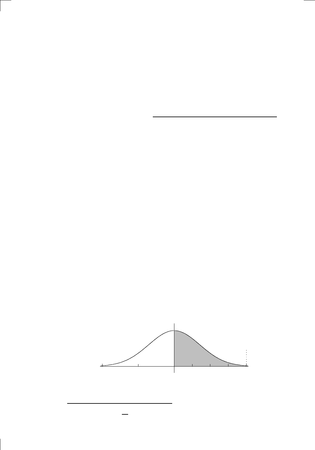
A p p e n d i x B
Estimating Integrals
Most of the time when we’ve looked at definite integrals, we’ve been used to
giving an exact answer by using antiderivatives and the Second Fundamental
Theorem. In real life, alas, finding antiderivatives in a useful form can be
difficult or impossible. Sometimes the best you can do is find an approxi-
mation to the value of your integral. So we’ll look at three techniques for
estimating definite integrals: strips, the trapezoidal rule, and Simpson’s rule.
In summary, here’s the plan for this final appendix:
• estimating definite integrals using strips, the trapezoidal rule, and Simp-
son’s rule; and
• estimating the error in the above approximations.
B.1 Estimating Integrals Using Strips
Here’s a perfectly reasonable definite integral:
Z
2
0
e
−x
2
dx.
It corresponds to the area of the region bounded by the x-axis, the curve
y = e
−x
2
, and the lines x = 0 and x = 2, like this:
PSfrag
replacements
(
a, b)
[
a, b]
(
a, b]
[
a, b)
(
a, ∞)
[
a, ∞)
(
−∞, b)
(
−∞, b]
(
−∞, ∞)
{
x : a < x < b}
{
x : a ≤ x ≤ b}
{
x : a < x ≤ b}
{
x : a ≤ x < b}
{
x : x ≥ a}
{
x : x > a}
{
x : x ≤ b}
{
x : x < b}
R
a
b
shado
w
0
1
4
−
2
3
−
3
g(
x) = x
2
f(
x) = x
3
g(
x) = x
2
f(
x) = x
3
mirror
(y = x)
f
−
1
(x) =
3
√
x
y = h
(x)
y = h
−
1
(x)
y =
(x − 1)
2
−
1
x
Same
height
−
x
Same
length,
opp
osite signs
y = −
2x
−
2
1
y =
1
2
x − 1
2
−
1
y =
2
x
y =
10
x
y =
2
−x
y =
log
2
(x)
4
3
units
mirror
(x-axis)
y = |
x|
y = |
log
2
(x)|
θ radians
θ units
30
◦
=
π
6
45
◦
=
π
4
60
◦
=
π
3
120
◦
=
2
π
3
135
◦
=
3
π
4
150
◦
=
5
π
6
90
◦
=
π
2
180
◦
= π
210
◦
=
7
π
6
225
◦
=
5
π
4
240
◦
=
4
π
3
270
◦
=
3
π
2
300
◦
=
5
π
3
315
◦
=
7
π
4
330
◦
=
11
π
6
0
◦
=
0 radians
θ
hyp
otenuse
opp
osite
adjacen
t
0
(≡ 2π)
π
2
π
3
π
2
I
I
I
I
II
IV
θ
(
x, y)
x
y
r
7
π
6
reference
angle
reference
angle =
π
6
sin
+
sin −
cos
+
cos −
tan
+
tan −
A
S
T
C
7
π
4
9
π
13
5
π
6
(this
angle is
5π
6
clo
ckwise)
1
2
1
2
3
4
5
6
0
−
1
−
2
−
3
−
4
−
5
−
6
−
3π
−
5
π
2
−
2π
−
3
π
2
−
π
−
π
2
3
π
3
π
5
π
2
2
π
3
π
2
π
π
2
y =
sin(x)
1
0
−
1
−
3π
−
5
π
2
−
2π
−
3
π
2
−
π
−
π
2
3
π
5
π
2
2
π
2
π
3
π
2
π
π
2
y =
sin(x)
y =
cos(x)
−
π
2
π
2
y =
tan(x), −
π
2
<
x <
π
2
0
−
π
2
π
2
y =
tan(x)
−
2π
−
3π
−
5
π
2
−
3
π
2
−
π
−
π
2
π
2
3
π
3
π
5
π
2
2
π
3
π
2
π
y =
sec(x)
y =
csc(x)
y =
cot(x)
y = f(
x)
−
1
1
2
y = g(
x)
3
y = h
(x)
4
5
−
2
f(
x) =
1
x
g(
x) =
1
x
2
etc.
0
1
π
1
2
π
1
3
π
1
4
π
1
5
π
1
6
π
1
7
π
g(
x) = sin
1
x
1
0
−
1
L
10
100
200
y =
π
2
y = −
π
2
y =
tan
−1
(x)
π
2
π
y =
sin(
x)
x
,
x > 3
0
1
−
1
a
L
f(
x) = x sin (1/x)
(0 <
x < 0.3)
h
(x) = x
g(
x) = −x
a
L
lim
x
→a
+
f(x) = L
lim
x
→a
+
f(x) = ∞
lim
x
→a
+
f(x) = −∞
lim
x
→a
+
f(x) DNE
lim
x
→a
−
f(x) = L
lim
x
→a
−
f(x) = ∞
lim
x
→a
−
f(x) = −∞
lim
x
→a
−
f(x) DNE
M
}
lim
x
→a
−
f(x) = M
lim
x
→a
f(x) = L
lim
x
→a
f(x) DNE
lim
x
→∞
f(x) = L
lim
x
→∞
f(x) = ∞
lim
x
→∞
f(x) = −∞
lim
x
→∞
f(x) DNE
lim
x
→−∞
f(x) = L
lim
x
→−∞
f(x) = ∞
lim
x
→−∞
f(x) = −∞
lim
x
→−∞
f(x) DNE
lim
x →a
+
f(
x) = ∞
lim
x →a
+
f(
x) = −∞
lim
x →a
−
f(
x) = ∞
lim
x →a
−
f(
x) = −∞
lim
x →a
f(
x) = ∞
lim
x →a
f(
x) = −∞
lim
x →a
f(
x) DNE
y = f (
x)
a
y =
|
x|
x
1
−
1
y =
|
x + 2|
x +
2
1
−
1
−
2
1
2
3
4
a
a
b
y = x sin
1
x
y = x
y = −
x
a
b
c
d
C
a
b
c
d
−
1
0
1
2
3
time
y
t
u
(
t, f(t))
(
u, f(u))
time
y
t
u
y
x
(
x, f(x))
y = |
x|
(
z, f(z))
z
y = f(
x)
a
tangen
t at x = a
b
tangen
t at x = b
c
tangen
t at x = c
y = x
2
tangen
t
at x = −
1
u
v
uv
u +
∆u
v +
∆v
(
u + ∆u)(v + ∆v)
∆
u
∆
v
u
∆v
v∆
u
∆
u∆v
y = f(
x)
1
2
−
2
y = |
x
2
− 4|
y = x
2
− 4
y = −
2x + 5
y = g(
x)
1
2
3
4
5
6
7
8
9
0
−
1
−
2
−
3
−
4
−
5
−
6
y = f (
x)
3
−
3
3
−
3
0
−
1
2
easy
hard
flat
y = f
0
(
x)
3
−
3
0
−
1
2
1
−
1
y =
sin(x)
y = x
x
A
B
O
1
C
D
sin(
x)
tan(
x)
y =
sin(
x)
x
π
2
π
1
−
1
x =
0
a =
0
x
> 0
a
> 0
x
< 0
a
< 0
rest
position
+
−
y = x
2
sin
1
x
N
A
B
H
a
b
c
O
H
A
B
C
D
h
r
R
θ
1000
2000
α
β
p
h
y = g(
x) = log
b
(x)
y = f(
x) = b
x
y = e
x
5
10
1
2
3
4
0
−
1
−
2
−
3
−
4
y =
ln(x)
y =
cosh(x)
y =
sinh(x)
y =
tanh(x)
y =
sech(x)
y =
csch(x)
y =
coth(x)
1
−
1
y = f(
x)
original
function
in
verse function
slop
e = 0 at (x, y)
slop
e is infinite at (y, x)
−
108
2
5
1
2
1
2
3
4
5
6
0
−
1
−
2
−
3
−
4
−
5
−
6
−
3π
−
5
π
2
−
2π
−
3
π
2
−
π
−
π
2
3
π
3
π
5
π
2
2
π
3
π
2
π
π
2
y =
sin(x)
1
0
−
1
−
3π
−
5
π
2
−
2π
−
3
π
2
−
π
−
π
2
3
π
5
π
2
2
π
2
π
3
π
2
π
π
2
y =
sin(x)
y =
sin(x), −
π
2
≤ x ≤
π
2
−
2
−
1
0
2
π
2
−
π
2
y =
sin
−1
(x)
y =
cos(x)
π
π
2
y =
cos
−1
(x)
−
π
2
1
x
α
β
y =
tan(x)
y =
tan(x)
1
y =
tan
−1
(x)
y =
sec(x)
y =
sec
−1
(x)
y =
csc
−1
(x)
y =
cot
−1
(x)
1
y =
cosh
−1
(x)
y =
sinh
−1
(x)
y =
tanh
−1
(x)
y =
sech
−1
(x)
y =
csch
−1
(x)
y =
coth
−1
(x)
(0
, 3)
(2
, −1)
(5
, 2)
(7
, 0)
(
−1, 44)
(0
, 1)
(1
, −12)
(2
, 305)
y =
1
2
(2
, 3)
y = f(
x)
y = g(
x)
a
b
c
a
b
c
s
c
0
c
1
(
a, f(a))
(
b, f(b))
1
2
1
2
3
4
5
6
0
−
1
−
2
−
3
−
4
−
5
−
6
−
3π
−
5
π
2
−
2π
−
3
π
2
−
π
−
π
2
3
π
3
π
5
π
2
2
π
3
π
2
π
π
2
y =
sin(x)
1
0
−
1
−
3π
−
5
π
2
−
2π
−
3
π
2
−
π
−
π
2
3
π
5
π
2
2
π
2
π
3
π
2
π
π
2
c
OR
Lo
cal maximum
Lo
cal minimum
Horizon
tal point of inflection
1
e
y = f
0
(
x)
y = f (
x) = x ln(x)
−
1
e
?
y = f(
x) = x
3
y = g(
x) = x
4
x
f(
x)
−
3
−
2
−
1
0
1
2
1
2
3
4
+
−
?
1
5
6
3
f
0
(
x)
2 −
1
2
√
6
2
+
1
2
√
6
f
00
(
x)
7
8
g
00
(
x)
f
00
(
x)
0
y =
(
x − 3)(x − 1)
2
x
3
(
x + 2)
y = x ln
(x)
1
e
−
1
e
5
−
108
2
α
β
2 −
1
2
√
6
2
+
1
2
√
6
y = x
2
(
x − 5)
3
−
e
−
1/2
√
3
e
−
1/2
√
3
−
e
−3/2
e
−
3/2
−
1
√
3
1
√
3
−
1
1
y = xe
−
3x
2
/2
y =
x
3
− 6
x
2
+ 13x − 8
x
28
2
600
500
400
300
200
100
0
−
100
−
200
−
300
−
400
−
500
−
600
0
10
−
10
5
−
5
20
−
20
15
−
15
0
4
5
6
x
P
0
(
x)
+
−
−
existing
fence
new
fence
enclosure
A
h
b
H
99
100
101
h
dA/dh
r
h
1
2
7
shallo
w
deep
LAND
SEA
N
y
z
s
t
3
11
9
L
(11)
√
11
y = L
(x)
y = f (
x)
11
y = L
(x)
y = f(
x)
F
P
a
a +
∆x
f(
a + ∆x)
L
(a + ∆x)
f(
a)
error
d
f
∆
x
a
b
y = f(
x)
true
zero
starting
approximation
b
etter approximation
v
t
3
5
50
40
60
4
20
30
25
t
1
t
2
t
3
t
4
t
n
−2
t
n
−1
t
0
= a
t
n
= b
v
1
v
2
v
3
v
4
v
n
−1
v
n
−
30
6
30
|
v|
a
b
p
q
c
v(
c)
v(
c
1
)
v(
c
2
)
v(
c
3
)
v(
c
4
)
v(
c
5
)
v(
c
6
)
t
1
t
2
t
3
t
4
t
5
c
1
c
2
c
3
c
4
c
5
c
6
t
0
=
a
t
6
=
b
t
16
=
b
t
10
=
b
a
b
x
y
y = f(
x)
1
2
y = x
5
0
−
2
y =
1
a
b
y =
sin(x)
π
−
π
0
−
1
−
2
0
2
4
y = x
2
0
1
2
3
4
2
n
4
n
6
n
2(
n−2)
n
2(
n−1)
n
2
n
n
=
2
width
of each interval =
2
n
−
2
1
3
0
I
I
I
I
II
IV
4
y
dx
y = −
x
2
− 2x + 3
3
−
5
y = |−
x
2
− 2x + 3|
I
I
I
I
Ia
5
3
0
1
2
a
b
y = f (
x)
y = g(
x)
y = x
2
a
b
5
3
0
1
2
y =
√
x
2
√
2
2
2
dy
x
2
a
b
y = f(
x)
y = g(
x)
M
m
1
2
−
1
−
2
0
y = e
−
x
2
1
2
e
−
1/4
f
a
v
y = f
a
v
c
A
M
0
1
2
a
b
x
t
y = f(
t)
F (
x )
y = f(
t)
F (
x + h)
x + h
F (
x + h) − F (x)
f(
x)
1
2
y =
sin(x)
π
−
π
−
1
−
2
y =
1
x
y = x
2
1
2
1
−
1
y =
ln|x|
θ
a
x
a
x
p
a
2
− x
2
3
x
p
9 − x
2
p
x
2
+ a
2
x
a
p
x
2
+ 15
x
√
15
x
p
x
2
− a
2
a
x
p
x
2
− 4
2
x
−
p
x
2
− a
2
a
x
−
p
x
2
− 4
2
y = f(
x)
a
b
a + ε
ε
Z
b
a
+ε
f(x) dx
small
ev
en smaller
y = g(
x)
infinite
area
finite
area
1
y =
1
x
y =
1
x
p
, p
< 1 (typical)
y =
1
x
p
, p
> 1 (typical)
a
1
a
2
a
3
a
4
a
5
a
6
a
7
a
8
1
2
3
4
5
6
7
8
n
a
n
x
y
y = f(
x)
(
a, f(a))
a
−
1
0
1
a
6
1
2
7
1
2
7
?
−
2
−
1
−
2
t =
0
t = π
/6
t = π
/4
t = π
/3
t = π
/2
3
0
t = −
2
t = −
3/2
t = ±
1
t = −
1/2
t =
0
t =
1/2
t =
3/2
t =
2
12
−
12
θ
r
P
θ
r
P
11
π
6
2
(
−1, −1)
wrong
point
π
4
5
π
4
√
2
(0
, 1)
(0
, −3)
(
−2, 0)
π
2
3
π
2
π
r =
3 sin(θ)
3
π
2
θ
2
π
1
0
−
1
−
2
−
3
0
3
2
−
3
2
0
r =
1 + 2 cos(θ)
2
π
3
4
π
3
0
π
0
pi
−
3
2
3
π
2
1
2
3
0
−
1
−
2
−
3
0 ≤ θ ≤
2
π
3
0 ≤ θ ≤ π
0 ≤ θ ≤ 2
π
r =
1 + cos(θ)
r =
1 +
3
4
cos(
θ)
−
1
4
r =
sin(2θ)
r =
sin(3θ)
r =
1
π
θ
0 ≤ θ ≤ 4
π
r =
2
1
+ sin(θ)
−
π
4
≤ θ ≤
5
π
4
0 ≤ θ ≤ 2
π
0 ≤ θ ≤ π
−
4
−5
4
5
f(θ)
f(θ + dθ)
θ
dθ
θ + dθ
approximating region
exact region
0 ≤ θ ≤ 2π
r = |1 + 2 cos(θ)|
2i
2 − 3i
−1
θ = 0
θ =
π
4
θ =
π
2
θ =
2π
3
θ = π
θ =
13π
12
θ =
3π
2
θ =
7π
4
1 = e
0
e
i
π
4
i = e
i
π
2
e
i
2π
3
−1 = e
iπ
e
i
13π
12
−i = e
i
3π
2
e
i
7π
4
i
−i
1
θ
1 − i
2i
−2i
2
−2
6i
−6i
6
−6
−
√
3
R
ϕ
2
1/5
θ =
π
6
θ =
17π
30
θ =
29π
30
θ =
41π
30
θ =
53π
30
z
0
z
1
z
2
z
3
z
4
−
√
3
2
√
3
2
1
2
i
−i
19π
6
−i
7π
6
i
5π
6
i
17π
6
i
29π
6
ln(2)
−
7π
4
−
3π
4
π
4
5π
4
9π
4
3
2
i
0
1
2
3
4
dx
y
x
y =
p
1 − (x − 3)
2
2πx
a
b
y = f(x)
A
B
y =
√
x
1
y = 2x
3
y = x
4
(2, 16)
−5
5
6
y = h
y−h
h−y
x = h
y
x−h
radius of shell = x−h
h−x
radius of shell = h−x
8
P
h
P
(slice)
(axis)
l
L
1
2
Base
Cross-section
Area = A
Area = A(x)
y = e
x
A
B
dx
dy
x + dx
a
b
p
(dx)
2
+ (dy)
2
P
t
600000
500000
400000
300000
200000
100000
−100000
−200000
−300000
−400000
−500000
−600000
0
1
2
3
4
5
6
7
L
ε
L + ε
L − ε
a
M
a + δ
a − δ
your move
my move
N
M
a + δ
a − δ
your move
my move
FIRST MOVE
SECOND MOVE
L + ε
L − ε
1
−1
L −
1
2
L +
1
2
L = 0
L = −
1
4
L =
7
8
L = 0
b
each segment is either the right half
or the left half of the one below it
infinitely many marked points
lie below each segment
0
1
1
2
−1
−2
y = e
−x
2
Finding an area like this might seem a little technical, but it’s actually in-
credibly useful. The above curve is commonly known as a bell-shaped curve,
∗
∗
Technically the bell-shaped curve, or normal distribution, is actually given by the
equation y = e
−x
2
/2
/
√
2π.
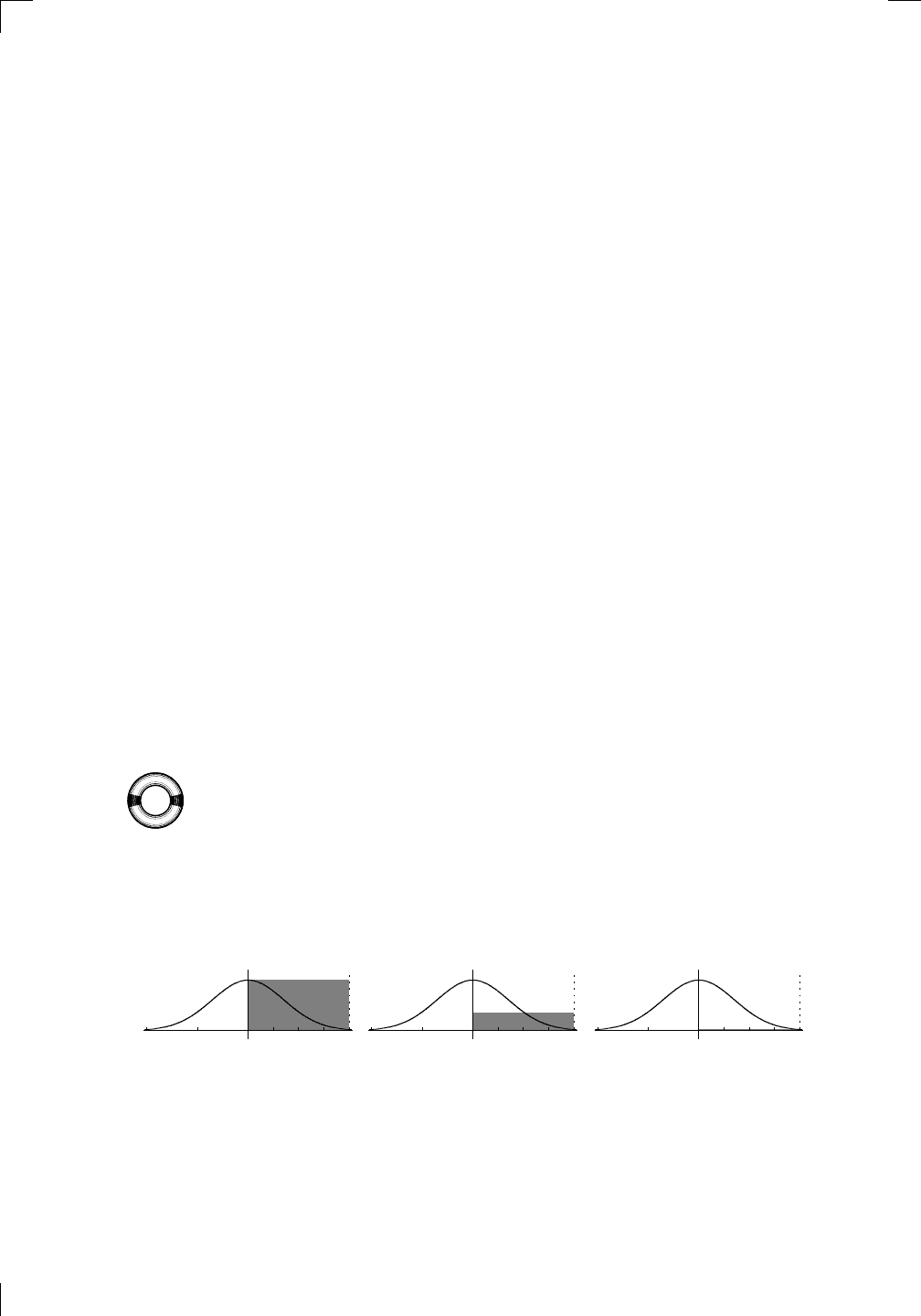
704 • Estimating Integrals
and it is fundamental in the study of probability theory. So it’s especially
annoying that there’s no nice, simple way to write down the antiderivative
Z
e
−x
2
dx.
Actually, you can use Maclaurin series to express this integral as an infinite
series, but that’s not so nice or simple. The cold, hard reality of the situation
is that there’s no way to write down the exact value of the definite integral at
the beginning of this section in a simple, closed form. (We already discussed
this point in Section 16.5.1 of Chapter 16.)
On the other hand, we can find an approximate value for the integral—
an estimate, if you prefer—by using the definition of the Riemann integral.
Indeed, in Section 16.2 of Chapter 16, we looked at partitions, meshes, and
Riemann sums. Since the integral is the limit of Riemann sums, we can get
an approximation simply by not taking the limit. So, to estimate the integral
Z
b
a
f(x) dx,
you can chop up the interval [a, b] into a partition of the form
a = x
0
< x
1
< ··· < x
n−1
< x
n
= b,
then choose a point c
1
in [x
0
, x
1
], a point c
2
in [x
1
, x
2
], and so on until you
choose c
n
in [x
n−1
, x
n
]. At that point, you’re ready to write
Z
b
a
f(x) dx
∼
=
n
X
j=1
f(c
j
)(x
j
− x
j−1
).
This just says that the integral is approximately equal to one of its Riemann
sums.
It all seems pretty abstract. Let’s see how it works in the case of our above
PSfrag
replacements
(
a, b)
[
a, b]
(
a, b]
[
a, b)
(
a, ∞)
[
a, ∞)
(
−∞, b)
(
−∞, b]
(
−∞, ∞)
{
x : a < x < b}
{
x : a ≤ x ≤ b}
{
x : a < x ≤ b}
{
x : a ≤ x < b}
{
x : x ≥ a}
{
x : x > a}
{
x : x ≤ b}
{
x : x < b}
R
a
b
shado
w
0
1
4
−
2
3
−
3
g(
x) = x
2
f(
x) = x
3
g(
x) = x
2
f(
x) = x
3
mirror
(y = x)
f
−
1
(x) =
3
√
x
y = h
(x)
y = h
−
1
(x)
y =
(x − 1)
2
−
1
x
Same
height
−
x
Same
length,
opp
osite signs
y = −
2x
−
2
1
y =
1
2
x − 1
2
−
1
y =
2
x
y =
10
x
y =
2
−x
y =
log
2
(x)
4
3
units
mirror
(x-axis)
y = |
x|
y = |
log
2
(x)|
θ radians
θ units
30
◦
=
π
6
45
◦
=
π
4
60
◦
=
π
3
120
◦
=
2
π
3
135
◦
=
3
π
4
150
◦
=
5
π
6
90
◦
=
π
2
180
◦
= π
210
◦
=
7
π
6
225
◦
=
5
π
4
240
◦
=
4
π
3
270
◦
=
3
π
2
300
◦
=
5
π
3
315
◦
=
7
π
4
330
◦
=
11
π
6
0
◦
=
0 radians
θ
hyp
otenuse
opp
osite
adjacen
t
0
(≡ 2π)
π
2
π
3
π
2
I
I
I
I
II
IV
θ
(
x, y)
x
y
r
7
π
6
reference
angle
reference
angle =
π
6
sin
+
sin −
cos
+
cos −
tan
+
tan −
A
S
T
C
7
π
4
9
π
13
5
π
6
(this
angle is
5π
6
clo
ckwise)
1
2
1
2
3
4
5
6
0
−
1
−
2
−
3
−
4
−
5
−
6
−
3π
−
5
π
2
−
2π
−
3
π
2
−
π
−
π
2
3
π
3
π
5
π
2
2
π
3
π
2
π
π
2
y =
sin(x)
1
0
−
1
−
3π
−
5
π
2
−
2π
−
3
π
2
−
π
−
π
2
3
π
5
π
2
2
π
2
π
3
π
2
π
π
2
y =
sin(x)
y =
cos(x)
−
π
2
π
2
y =
tan(x), −
π
2
<
x <
π
2
0
−
π
2
π
2
y =
tan(x)
−
2π
−
3π
−
5
π
2
−
3
π
2
−
π
−
π
2
π
2
3
π
3
π
5
π
2
2
π
3
π
2
π
y =
sec(x)
y =
csc(x)
y =
cot(x)
y = f(
x)
−
1
1
2
y = g(
x)
3
y = h
(x)
4
5
−
2
f(
x) =
1
x
g(
x) =
1
x
2
etc.
0
1
π
1
2
π
1
3
π
1
4
π
1
5
π
1
6
π
1
7
π
g(
x) = sin
1
x
1
0
−
1
L
10
100
200
y =
π
2
y = −
π
2
y =
tan
−1
(x)
π
2
π
y =
sin(
x)
x
,
x > 3
0
1
−
1
a
L
f(
x) = x sin (1/x)
(0 <
x < 0.3)
h
(x) = x
g(
x) = −x
a
L
lim
x
→a
+
f(x) = L
lim
x
→a
+
f(x) = ∞
lim
x
→a
+
f(x) = −∞
lim
x
→a
+
f(x) DNE
lim
x
→a
−
f(x) = L
lim
x
→a
−
f(x) = ∞
lim
x
→a
−
f(x) = −∞
lim
x
→a
−
f(x) DNE
M
}
lim
x
→a
−
f(x) = M
lim
x
→a
f(x) = L
lim
x
→a
f(x) DNE
lim
x
→∞
f(x) = L
lim
x
→∞
f(x) = ∞
lim
x
→∞
f(x) = −∞
lim
x
→∞
f(x) DNE
lim
x
→−∞
f(x) = L
lim
x
→−∞
f(x) = ∞
lim
x
→−∞
f(x) = −∞
lim
x
→−∞
f(x) DNE
lim
x →a
+
f(
x) = ∞
lim
x →a
+
f(
x) = −∞
lim
x →a
−
f(
x) = ∞
lim
x →a
−
f(
x) = −∞
lim
x →a
f(
x) = ∞
lim
x →a
f(
x) = −∞
lim
x →a
f(
x) DNE
y = f (
x)
a
y =
|
x|
x
1
−
1
y =
|
x + 2|
x +
2
1
−
1
−
2
1
2
3
4
a
a
b
y = x sin
1
x
y = x
y = −
x
a
b
c
d
C
a
b
c
d
−
1
0
1
2
3
time
y
t
u
(
t, f(t))
(
u, f(u))
time
y
t
u
y
x
(
x, f(x))
y = |
x|
(
z, f(z))
z
y = f(
x)
a
tangen
t at x = a
b
tangen
t at x = b
c
tangen
t at x = c
y = x
2
tangen
t
at x = −
1
u
v
uv
u +
∆u
v +
∆v
(
u + ∆u)(v + ∆v)
∆
u
∆
v
u
∆v
v∆
u
∆
u∆v
y = f(
x)
1
2
−
2
y = |
x
2
− 4|
y = x
2
− 4
y = −
2x + 5
y = g(
x)
1
2
3
4
5
6
7
8
9
0
−
1
−
2
−
3
−
4
−
5
−
6
y = f (
x)
3
−
3
3
−
3
0
−
1
2
easy
hard
flat
y = f
0
(
x)
3
−
3
0
−
1
2
1
−
1
y =
sin(x)
y = x
x
A
B
O
1
C
D
sin(
x)
tan(
x)
y =
sin(
x)
x
π
2
π
1
−
1
x =
0
a =
0
x
> 0
a
> 0
x
< 0
a
< 0
rest
position
+
−
y = x
2
sin
1
x
N
A
B
H
a
b
c
O
H
A
B
C
D
h
r
R
θ
1000
2000
α
β
p
h
y = g(
x) = log
b
(x)
y = f(
x) = b
x
y = e
x
5
10
1
2
3
4
0
−
1
−
2
−
3
−
4
y =
ln(x)
y =
cosh(x)
y =
sinh(x)
y =
tanh(x)
y =
sech(x)
y =
csch(x)
y =
coth(x)
1
−
1
y = f(
x)
original
function
in
verse function
slop
e = 0 at (x, y)
slop
e is infinite at (y, x)
−
108
2
5
1
2
1
2
3
4
5
6
0
−
1
−
2
−
3
−
4
−
5
−
6
−
3π
−
5
π
2
−
2π
−
3
π
2
−
π
−
π
2
3
π
3
π
5
π
2
2
π
3
π
2
π
π
2
y =
sin(x)
1
0
−
1
−
3π
−
5
π
2
−
2π
−
3
π
2
−
π
−
π
2
3
π
5
π
2
2
π
2
π
3
π
2
π
π
2
y =
sin(x)
y =
sin(x), −
π
2
≤ x ≤
π
2
−
2
−
1
0
2
π
2
−
π
2
y =
sin
−1
(x)
y =
cos(x)
π
π
2
y =
cos
−1
(x)
−
π
2
1
x
α
β
y =
tan(x)
y =
tan(x)
1
y =
tan
−1
(x)
y =
sec(x)
y =
sec
−1
(x)
y =
csc
−1
(x)
y =
cot
−1
(x)
1
y =
cosh
−1
(x)
y =
sinh
−1
(x)
y =
tanh
−1
(x)
y =
sech
−1
(x)
y =
csch
−1
(x)
y =
coth
−1
(x)
(0
, 3)
(2
, −1)
(5
, 2)
(7
, 0)
(
−1, 44)
(0
, 1)
(1
, −12)
(2
, 305)
y =
1
2
(2
, 3)
y = f(
x)
y = g(
x)
a
b
c
a
b
c
s
c
0
c
1
(
a, f(a))
(
b, f(b))
1
2
1
2
3
4
5
6
0
−
1
−
2
−
3
−
4
−
5
−
6
−
3π
−
5
π
2
−
2π
−
3
π
2
−
π
−
π
2
3
π
3
π
5
π
2
2
π
3
π
2
π
π
2
y =
sin(x)
1
0
−
1
−
3π
−
5
π
2
−
2π
−
3
π
2
−
π
−
π
2
3
π
5
π
2
2
π
2
π
3
π
2
π
π
2
c
OR
Lo
cal maximum
Lo
cal minimum
Horizon
tal point of inflection
1
e
y = f
0
(
x)
y = f (
x) = x ln(x)
−
1
e
?
y = f(
x) = x
3
y = g(
x) = x
4
x
f(
x)
−
3
−
2
−
1
0
1
2
1
2
3
4
+
−
?
1
5
6
3
f
0
(
x)
2 −
1
2
√
6
2
+
1
2
√
6
f
00
(
x)
7
8
g
00
(
x)
f
00
(
x)
0
y =
(
x − 3)(x − 1)
2
x
3
(
x + 2)
y = x ln
(x)
1
e
−
1
e
5
−
108
2
α
β
2 −
1
2
√
6
2
+
1
2
√
6
y = x
2
(
x − 5)
3
−
e
−
1/2
√
3
e
−
1/2
√
3
−
e
−3/2
e
−
3/2
−
1
√
3
1
√
3
−
1
1
y = xe
−
3x
2
/2
y =
x
3
− 6
x
2
+ 13x − 8
x
28
2
600
500
400
300
200
100
0
−
100
−
200
−
300
−
400
−
500
−
600
0
10
−
10
5
−
5
20
−
20
15
−
15
0
4
5
6
x
P
0
(
x)
+
−
−
existing
fence
new
fence
enclosure
A
h
b
H
99
100
101
h
dA/dh
r
h
1
2
7
shallo
w
deep
LAND
SEA
N
y
z
s
t
3
11
9
L
(11)
√
11
y = L
(x)
y = f (
x)
11
y = L
(x)
y = f(
x)
F
P
a
a +
∆x
f(
a + ∆x)
L
(a + ∆x)
f(
a)
error
d
f
∆
x
a
b
y = f(
x)
true
zero
starting
approximation
b
etter approximation
v
t
3
5
50
40
60
4
20
30
25
t
1
t
2
t
3
t
4
t
n
−2
t
n
−1
t
0
= a
t
n
= b
v
1
v
2
v
3
v
4
v
n
−1
v
n
−
30
6
30
|
v|
a
b
p
q
c
v(
c)
v(
c
1
)
v(
c
2
)
v(
c
3
)
v(
c
4
)
v(
c
5
)
v(
c
6
)
t
1
t
2
t
3
t
4
t
5
c
1
c
2
c
3
c
4
c
5
c
6
t
0
=
a
t
6
=
b
t
16
=
b
t
10
=
b
a
b
x
y
y = f(
x)
1
2
y = x
5
0
−
2
y =
1
a
b
y =
sin(x)
π
−
π
0
−
1
−
2
0
2
4
y = x
2
0
1
2
3
4
2
n
4
n
6
n
2(
n−2)
n
2(
n−1)
n
2
n
n
=
2
width
of each interval =
2
n
−
2
1
3
0
I
I
I
I
II
IV
4
y
dx
y = −
x
2
− 2x + 3
3
−
5
y = |−
x
2
− 2x + 3|
I
I
I
I
Ia
5
3
0
1
2
a
b
y = f (
x)
y = g(
x)
y = x
2
a
b
5
3
0
1
2
y =
√
x
2
√
2
2
2
dy
x
2
a
b
y = f(
x)
y = g(
x)
M
m
1
2
−
1
−
2
0
y = e
−
x
2
1
2
e
−
1/4
f
a
v
y = f
a
v
c
A
M
0
1
2
a
b
x
t
y = f (
t)
F (
x )
y = f (
t)
F (
x + h)
x + h
F (
x + h) − F (x)
f(
x)
1
2
y =
sin(x)
π
−
π
−
1
−
2
y =
1
x
y = x
2
1
2
1
−
1
y =
ln|x|
θ
a
x
a
x
p
a
2
− x
2
3
x
p
9 − x
2
p
x
2
+ a
2
x
a
p
x
2
+ 15
x
√
15
x
p
x
2
− a
2
a
x
p
x
2
− 4
2
x
−
p
x
2
− a
2
a
x
−
p
x
2
− 4
2
y = f(
x)
a
b
a + ε
ε
Z
b
a
+ε
f(x) dx
small
ev
en smaller
y = g(
x)
infinite
area
finite
area
1
y =
1
x
y =
1
x
p
, p
< 1 (typical)
y =
1
x
p
, p
> 1 (typical)
a
1
a
2
a
3
a
4
a
5
a
6
a
7
a
8
1
2
3
4
5
6
7
8
n
a
n
x
y
y = f(
x)
(
a, f(a))
a
−
1
0
1
a
6
1
2
7
1
2
7
?
−
2
−
1
−
2
t =
0
t = π
/6
t = π
/4
t = π
/3
t = π
/2
3
0
t = −
2
t = −
3/2
t = ±
1
t = −
1/2
t =
0
t =
1/2
t =
3/2
t =
2
12
−
12
θ
r
P
θ
r
P
11
π
6
2
(
−1, −1)
wrong
point
π
4
5
π
4
√
2
(0
, 1)
(0
, −3)
(
−2, 0)
π
2
3
π
2
π
r =
3 sin(θ)
3
π
2
θ
2
π
1
0
−
1
−
2
−
3
0
3
2
−
3
2
0
r =
1 + 2 cos(θ)
2
π
3
4
π
3
0
π
0
pi
−
3
2
3
π
2
1
2
3
0
−
1
−
2
−
3
0 ≤ θ ≤
2
π
3
0 ≤ θ ≤ π
0 ≤ θ ≤ 2
π
r =
1 + cos(θ)
r =
1 +
3
4
cos(
θ)
−
1
4
r =
sin(2θ)
r =
sin(3θ)
r =
1
π
θ
0 ≤ θ ≤ 4
π
r =
2
1
+ sin(θ)
−
π
4
≤ θ ≤
5
π
4
0 ≤ θ ≤ 2
π
0 ≤ θ ≤ π
−
4
−
5
4
5
f(
θ)
f(
θ + dθ)
θ
dθ
θ + dθ
appro
ximating region
exact
region
0 ≤ θ ≤ 2
π
r = |
1 + 2 cos(θ)|
2i
2 − 3i
−1
θ = 0
θ =
π
4
θ =
π
2
θ =
2π
3
θ = π
θ =
13π
12
θ =
3π
2
θ =
7π
4
1 = e
0
e
i
π
4
i = e
i
π
2
e
i
2π
3
−1 = e
iπ
e
i
13π
12
−i = e
i
3π
2
e
i
7π
4
i
−i
1
θ
1 − i
2i
−2i
2
−2
6i
−6i
6
−6
−
√
3
R
ϕ
2
1/5
θ =
π
6
θ =
17π
30
θ =
29π
30
θ =
41π
30
θ =
53π
30
z
0
z
1
z
2
z
3
z
4
−
√
3
2
√
3
2
1
2
i
−i
19π
6
−i
7π
6
i
5π
6
i
17π
6
i
29π
6
ln(2)
−
7π
4
−
3π
4
π
4
5π
4
9π
4
3
2
i
0
1
2
3
4
dx
y
x
y =
p
1 − (x − 3)
2
2πx
a
b
y = f(x)
A
B
y =
√
x
1
y = 2x
3
y = x
4
(2, 16)
−5
5
6
y = h
y−h
h−y
x = h
y
x−h
radius of shell = x−h
h−x
radius of shell = h−x
8
P
h
P
(slice)
(axis)
l
L
1
2
Base
Cross-section
Area = A
Area = A(x)
y = e
x
A
B
dx
dy
x + dx
a
b
p
(dx)
2
+ (dy)
2
P
t
600000
500000
400000
300000
200000
100000
−100000
−200000
−300000
−400000
−500000
−600000
0
1
2
3
4
5
6
7
L
ε
L + ε
L − ε
a
M
a + δ
a − δ
your move
my move
N
M
a + δ
a − δ
your move
my move
FIRST MOVE
SECOND MOVE
L + ε
L − ε
1
−1
L −
1
2
L +
1
2
L = 0
L = −
1
4
L =
7
8
L = 0
b
each segment is either the right half
or the left half of the one below it
infinitely many marked points
lie below each segment
0
1
2
−1
−2
y = e
−x
2
example. We’re integrating from 0 to 2, so we need a partition of the integral
[0, 2]. The simplest partition of that interval is just the interval [0, 2], which
corresponds to the choices n = 1, x
0
= 0, and x
1
= 2. We just need to pick c
1
inside [0, 2]. The approximation we’ll end up with depends a lot on this choice!
For example, if you choose c
1
= 0, c
1
= 1, or c
1
= 2, then your approximations
will end up being the areas of the following regions, respectively:
PSfrag
replacements
(
a, b)
[
a, b]
(
a, b]
[
a, b)
(
a, ∞)
[
a, ∞)
(
−∞, b)
(
−∞, b]
(
−∞, ∞)
{
x : a < x < b}
{
x : a ≤ x ≤ b}
{
x : a < x ≤ b}
{
x : a ≤ x < b}
{
x : x ≥ a}
{
x : x > a}
{
x : x ≤ b}
{
x : x < b}
R
a
b
shado
w
0
1
4
−
2
3
−
3
g(
x) = x
2
f(
x) = x
3
g(
x) = x
2
f(
x) = x
3
mirror
(y = x)
f
−
1
(x) =
3
√
x
y = h
(x)
y = h
−
1
(x)
y =
(x − 1)
2
−
1
x
Same
height
−
x
Same
length,
opp
osite signs
y = −
2x
−
2
1
y =
1
2
x − 1
2
−
1
y =
2
x
y =
10
x
y =
2
−x
y =
log
2
(x)
4
3
units
mirror
(x-axis)
y = |
x|
y = |
log
2
(x)|
θ radians
θ units
30
◦
=
π
6
45
◦
=
π
4
60
◦
=
π
3
120
◦
=
2
π
3
135
◦
=
3
π
4
150
◦
=
5
π
6
90
◦
=
π
2
180
◦
= π
210
◦
=
7
π
6
225
◦
=
5
π
4
240
◦
=
4
π
3
270
◦
=
3
π
2
300
◦
=
5
π
3
315
◦
=
7
π
4
330
◦
=
11
π
6
0
◦
=
0 radians
θ
hyp
otenuse
opp
osite
adjacen
t
0
(≡ 2π)
π
2
π
3
π
2
I
I
I
I
II
IV
θ
(
x, y)
x
y
r
7
π
6
reference
angle
reference
angle =
π
6
sin
+
sin −
cos
+
cos −
tan
+
tan −
A
S
T
C
7
π
4
9
π
13
5
π
6
(this
angle is
5π
6
clo
ckwise)
1
2
1
2
3
4
5
6
0
−
1
−
2
−
3
−
4
−
5
−
6
−
3π
−
5
π
2
−
2π
−
3
π
2
−
π
−
π
2
3
π
3
π
5
π
2
2
π
3
π
2
π
π
2
y =
sin(x)
1
0
−
1
−
3π
−
5
π
2
−
2π
−
3
π
2
−
π
−
π
2
3
π
5
π
2
2
π
2
π
3
π
2
π
π
2
y =
sin(x)
y =
cos(x)
−
π
2
π
2
y =
tan(x), −
π
2
<
x <
π
2
0
−
π
2
π
2
y =
tan(x)
−
2π
−
3π
−
5
π
2
−
3
π
2
−
π
−
π
2
π
2
3
π
3
π
5
π
2
2
π
3
π
2
π
y =
sec(x)
y =
csc(x)
y =
cot(x)
y = f(
x)
−
1
1
2
y = g(
x)
3
y = h
(x)
4
5
−
2
f(
x) =
1
x
g(
x) =
1
x
2
etc.
0
1
π
1
2
π
1
3
π
1
4
π
1
5
π
1
6
π
1
7
π
g(
x) = sin
1
x
1
0
−
1
L
10
100
200
y =
π
2
y = −
π
2
y =
tan
−1
(x)
π
2
π
y =
sin
(x)
x
,
x > 3
0
1
−
1
a
L
f(
x) = x sin (1/x)
(0 <
x < 0.3)
h
(x) = x
g(
x) = −x
a
L
lim
x
→a
+
f(x) = L
lim
x
→a
+
f(x) = ∞
lim
x
→a
+
f(x) = −∞
lim
x
→a
+
f(x) DNE
lim
x
→a
−
f(x) = L
lim
x
→a
−
f(x) = ∞
lim
x
→a
−
f(x) = −∞
lim
x
→a
−
f(x) DNE
M
}
lim
x
→a
−
f(x) = M
lim
x
→a
f(x) = L
lim
x
→a
f(x) DNE
lim
x
→∞
f(x) = L
lim
x
→∞
f(x) = ∞
lim
x
→∞
f(x) = −∞
lim
x
→∞
f(x) DNE
lim
x
→−∞
f(x) = L
lim
x
→−∞
f(x) = ∞
lim
x
→−∞
f(x) = −∞
lim
x
→−∞
f(x) DNE
lim
x →a
+
f(
x) = ∞
lim
x →a
+
f(
x) = −∞
lim
x →a
−
f(
x) = ∞
lim
x →a
−
f(
x) = −∞
lim
x →a
f(
x) = ∞
lim
x →a
f(
x) = −∞
lim
x →a
f(
x) DNE
y = f (
x)
a
y =
|
x|
x
1
−
1
y =
|
x + 2|
x +
2
1
−
1
−
2
1
2
3
4
a
a
b
y = x sin
1
x
y = x
y = −
x
a
b
c
d
C
a
b
c
d
−
1
0
1
2
3
time
y
t
u
(
t, f(t))
(
u, f(u))
time
y
t
u
y
x
(
x, f(x))
y = |
x|
(
z, f(z))
z
y = f(
x)
a
tangen
t at x = a
b
tangen
t at x = b
c
tangen
t at x = c
y = x
2
tangen
t
at x = −
1
u
v
uv
u +
∆u
v +
∆v
(
u + ∆u)(v + ∆v)
∆
u
∆
v
u
∆v
v∆
u
∆
u∆v
y = f(
x)
1
2
−
2
y = |
x
2
− 4|
y = x
2
− 4
y = −
2x + 5
y = g(
x)
1
2
3
4
5
6
7
8
9
0
−
1
−
2
−
3
−
4
−
5
−
6
y = f(
x)
3
−
3
3
−
3
0
−
1
2
easy
hard
flat
y = f
0
(
x)
3
−
3
0
−
1
2
1
−
1
y =
sin(x)
y = x
x
A
B
O
1
C
D
sin(
x)
tan(
x)
y =
sin
(x)
x
π
2
π
1
−
1
x =
0
a =
0
x
> 0
a
> 0
x
< 0
a
< 0
rest
position
+
−
y = x
2
sin
1
x
N
A
B
H
a
b
c
O
H
A
B
C
D
h
r
R
θ
1000
2000
α
β
p
h
y = g(
x) = log
b
(x)
y = f (
x) = b
x
y = e
x
5
10
1
2
3
4
0
−
1
−
2
−
3
−
4
y =
ln(x)
y =
cosh(x)
y =
sinh(x)
y =
tanh(x)
y =
sech(x)
y =
csch(x)
y =
coth(x)
1
−
1
y = f(
x)
original
function
in
verse function
slop
e = 0 at (x, y)
slop
e is infinite at (y, x)
−
108
2
5
1
2
1
2
3
4
5
6
0
−
1
−
2
−
3
−
4
−
5
−
6
−
3π
−
5
π
2
−
2π
−
3
π
2
−
π
−
π
2
3
π
3
π
5
π
2
2
π
3
π
2
π
π
2
y =
sin(x)
1
0
−
1
−
3π
−
5
π
2
−
2π
−
3
π
2
−
π
−
π
2
3
π
5
π
2
2
π
2
π
3
π
2
π
π
2
y =
sin(x)
y =
sin(x), −
π
2
≤ x ≤
π
2
−
2
−
1
0
2
π
2
−
π
2
y =
sin
−1
(x)
y =
cos(x)
π
π
2
y =
cos
−1
(x)
−
π
2
1
x
α
β
y =
tan(x)
y =
tan(x)
1
y =
tan
−1
(x)
y =
sec(x)
y =
sec
−1
(x)
y =
csc
−1
(x)
y =
cot
−1
(x)
1
y =
cosh
−1
(x)
y =
sinh
−1
(x)
y =
tanh
−1
(x)
y =
sech
−1
(x)
y =
csch
−1
(x)
y =
coth
−1
(x)
(0
, 3)
(2
, −1)
(5
, 2)
(7
, 0)
(
−1, 44)
(0
, 1)
(1
, −12)
(2
, 305)
y =
1
2
(2
, 3)
y = f(
x)
y = g(
x)
a
b
c
a
b
c
s
c
0
c
1
(
a, f(a))
(
b, f(b))
1
2
1
2
3
4
5
6
0
−
1
−
2
−
3
−
4
−
5
−
6
−
3π
−
5
π
2
−
2π
−
3
π
2
−
π
−
π
2
3
π
3
π
5
π
2
2
π
3
π
2
π
π
2
y =
sin(x)
1
0
−
1
−
3π
−
5
π
2
−
2π
−
3
π
2
−
π
−
π
2
3
π
5
π
2
2
π
2
π
3
π
2
π
π
2
c
OR
Lo
cal maximum
Lo
cal minimum
Horizon
tal point of inflection
1
e
y = f
0
(
x)
y = f(
x) = x ln(x)
−
1
e
?
y = f (
x) = x
3
y = g(
x) = x
4
x
f(
x)
−
3
−
2
−
1
0
1
2
1
2
3
4
+
−
?
1
5
6
3
f
0
(
x)
2 −
1
2
√
6
2
+
1
2
√
6
f
00
(
x)
7
8
g
00
(
x)
f
00
(
x)
0
y =
(
x − 3)(x − 1)
2
x
3
(
x + 2)
y = x ln(
x)
1
e
−
1
e
5
−
108
2
α
β
2 −
1
2
√
6
2
+
1
2
√
6
y = x
2
(
x − 5)
3
−
e
−
1/2
√
3
e
−
1/2
√
3
−
e
−3/2
e
−
3/2
−
1
√
3
1
√
3
−
1
1
y = xe
−
3x
2
/2
y =
x
3
− 6
x
2
+ 13x − 8
x
28
2
600
500
400
300
200
100
0
−
100
−
200
−
300
−
400
−
500
−
600
0
10
−
10
5
−
5
20
−
20
15
−
15
0
4
5
6
x
P
0
(
x)
+
−
−
existing
fence
new
fence
enclosure
A
h
b
H
99
100
101
h
dA/dh
r
h
1
2
7
shallo
w
deep
LAND
SEA
N
y
z
s
t
3
11
9
L
(11)
√
11
y = L
(x)
y = f(
x)
11
y = L
(x)
y = f(
x)
F
P
a
a +
∆x
f(
a + ∆x)
L
(a + ∆x)
f(
a)
error
d
f
∆
x
a
b
y = f(
x)
true
zero
starting
approximation
b
etter approximation
v
t
3
5
50
40
60
4
20
30
25
t
1
t
2
t
3
t
4
t
n
−2
t
n
−1
t
0
= a
t
n
= b
v
1
v
2
v
3
v
4
v
n
−1
v
n
−
30
6
30
|
v|
a
b
p
q
c
v(
c)
v(
c
1
)
v(
c
2
)
v(
c
3
)
v(
c
4
)
v(
c
5
)
v(
c
6
)
t
1
t
2
t
3
t
4
t
5
c
1
c
2
c
3
c
4
c
5
c
6
t
0
=
a
t
6
=
b
t
16
=
b
t
10
=
b
a
b
x
y
y = f(
x)
1
2
y = x
5
0
−
2
y =
1
a
b
y =
sin(x)
π
−
π
0
−
1
−
2
0
2
4
y = x
2
0
1
2
3
4
2
n
4
n
6
n
2(
n−2)
n
2(
n−1)
n
2
n
n
=
2
width
of each interval =
2
n
−
2
1
3
0
I
I
I
I
II
IV
4
y
dx
y = −
x
2
− 2x + 3
3
−
5
y = |−
x
2
− 2x + 3|
I
I
I
I
Ia
5
3
0
1
2
a
b
y = f (
x)
y = g(
x)
y = x
2
a
b
5
3
0
1
2
y =
√
x
2
√
2
2
2
dy
x
2
a
b
y = f(
x)
y = g(
x)
M
m
1
2
−
1
−
2
0
y = e
−
x
2
1
2
e
−
1/4
f
a
v
y = f
a
v
c
A
M
0
1
2
a
b
x
t
y = f(
t)
F (
x )
y = f(
t)
F (
x + h )
x + h
F (
x + h) − F (x)
f(
x)
1
2
y =
sin(x)
π
−
π
−
1
−
2
y =
1
x
y = x
2
1
2
1
−
1
y =
ln|x|
θ
a
x
a
x
p
a
2
− x
2
3
x
p
9 − x
2
p
x
2
+ a
2
x
a
p
x
2
+ 15
x
√
15
x
p
x
2
− a
2
a
x
p
x
2
− 4
2
x
−
p
x
2
− a
2
a
x
−
p
x
2
− 4
2
y = f(
x)
a
b
a + ε
ε
Z
b
a
+ε
f(x) dx
small
ev
en smaller
y = g(
x)
infinite
area
finite
area
1
y =
1
x
y =
1
x
p
, p
< 1 (typical)
y =
1
x
p
, p
> 1 (typical)
a
1
a
2
a
3
a
4
a
5
a
6
a
7
a
8
1
2
3
4
5
6
7
8
n
a
n
x
y
y = f(
x)
(
a, f(a))
a
−
1
0
1
a
6
1
2
7
1
2
7
?
−
2
−
1
−
2
t =
0
t = π
/6
t = π
/4
t = π
/3
t = π
/2
3
0
t = −
2
t = −
3/2
t = ±
1
t = −
1/2
t =
0
t =
1/2
t =
3/2
t =
2
12
−
12
θ
r
P
θ
r
P
11
π
6
2
(
−1, −1)
wrong
point
π
4
5
π
4
√
2
(0
, 1)
(0
, −3)
(
−2, 0)
π
2
3
π
2
π
r =
3 sin(θ)
3
π
2
θ
2
π
1
0
−
1
−
2
−
3
0
3
2
−
3
2
0
r =
1 + 2 cos(θ)
2
π
3
4
π
3
0
π
0
pi
−
3
2
3
π
2
1
2
3
0
−
1
−
2
−
3
0 ≤ θ ≤
2
π
3
0 ≤ θ ≤ π
0 ≤ θ ≤ 2
π
r =
1 + cos(θ)
r =
1 +
3
4
cos
(θ)
−
1
4
r =
sin(2θ)
r =
sin(3θ)
r =
1
π
θ
0 ≤ θ ≤ 4
π
r =
2
1
+ sin(θ)
−
π
4
≤ θ ≤
5
π
4
0 ≤ θ ≤ 2
π
0 ≤ θ ≤ π
−
4
−
5
4
5
f(θ)
f(θ + dθ)
θ
dθ
θ + dθ
approximating region
exact region
0 ≤ θ ≤ 2π
r = |1 + 2 cos(θ)|
2i
2 − 3i
−1
θ = 0
θ =
π
4
θ =
π
2
θ =
2π
3
θ = π
θ =
13π
12
θ =
3π
2
θ =
7π
4
1 = e
0
e
i
π
4
i = e
i
π
2
e
i
2π
3
−1 = e
iπ
e
i
13π
12
−i = e
i
3π
2
e
i
7π
4
i
−i
1
θ
1 − i
2i
−2i
2
−2
6i
−6i
6
−6
−
√
3
R
ϕ
2
1/5
θ =
π
6
θ =
17π
30
θ =
29π
30
θ =
41π
30
θ =
53π
30
z
0
z
1
z
2
z
3
z
4
−
√
3
2
√
3
2
1
2
i
−i
19π
6
−i
7π
6
i
5π
6
i
17π
6
i
29π
6
ln(2)
−
7π
4
−
3π
4
π
4
5π
4
9π
4
3
2
i
0
1
2
3
4
dx
y
x
y =
p
1 − (x − 3)
2
2πx
a
b
y = f(x)
A
B
y =
√
x
1
y = 2x
3
y = x
4
(2, 16)
−5
5
6
y = h
y−h
h−y
x = h
y
x−h
radius of shell = x−h
h−x
radius of shell = h−x
8
P
h
P
(slice)
(axis)
l
L
1
2
Base
Cross-section
Area = A
Area = A(x)
y = e
x
A
B
dx
dy
x + dx
a
b
p
(dx)
2
+ (dy)
2
P
t
600000
500000
400000
300000
200000
100000
−100000
−200000
−300000
−400000
−500000
−600000
0
1
2
3
4
5
6
7
L
ε
L + ε
L − ε
a
M
a + δ
a − δ
your move
my move
N
M
a + δ
a − δ
your move
my move
FIRST MOVE
SECOND MOVE
L + ε
L − ε
1
−1
L −
1
2
L +
1
2
L = 0
L = −
1
4
L =
7
8
L = 0
b
each segment is either the right half
or the left half of the one below it
infinitely many marked points
lie below each segment
0
1
2
−1
−2
y = e
−x
2
0
0
0
111
1
1
12
2
2
−1
−1
−1
−2
−2
−2
The first one is clearly a huge overestimate, while the third one is an under-
estimate. The middle isn’t so bad, but still not perfect. In order to work out
the values of these three estimates, we’ll use the formula:
Z
2
0
e
−x
2
dx
∼
=
n
X
j=1
f(c
j
)(x
j
− x
j−1
).
Section B.1.1: Evenly spaced partitions • 705
Replacing n by 1, f(c
1
) by e
−c
2
1
, x
0
by 0, and x
1
by 2, we get
Z
2
0
e
−x
2
dx
∼
=
e
−c
2
1
(2 − 0) = 2e
−c
2
1
.
When c
1
is 0, 1, and 2, these values are 2, 2/e
∼
=
0.736, and 2/e
4
∼
=
0.037,
respectively. As you can see, there’s a lot of difference between these three
estimates!
Now let’s see if we can do better by using more strips. Suppose we take a
PSfrag
replacements
(
a, b)
[
a, b]
(
a, b]
[
a, b)
(
a, ∞)
[
a, ∞)
(
−∞, b)
(
−∞, b]
(
−∞, ∞)
{
x : a < x < b}
{
x : a ≤ x ≤ b}
{
x : a < x ≤ b}
{
x : a ≤ x < b}
{
x : x ≥ a}
{
x : x > a}
{
x : x ≤ b}
{
x : x < b}
R
a
b
shado
w
0
1
4
−
2
3
−
3
g(
x) = x
2
f(
x) = x
3
g(
x) = x
2
f(
x) = x
3
mirror
(y = x)
f
−
1
(x) =
3
√
x
y = h
(x)
y = h
−
1
(x)
y =
(x − 1)
2
−
1
x
Same
height
−
x
Same
length,
opp
osite signs
y = −
2x
−
2
1
y =
1
2
x − 1
2
−
1
y =
2
x
y =
10
x
y =
2
−x
y =
log
2
(x)
4
3
units
mirror
(x-axis)
y = |
x|
y = |
log
2
(x)|
θ radians
θ units
30
◦
=
π
6
45
◦
=
π
4
60
◦
=
π
3
120
◦
=
2
π
3
135
◦
=
3
π
4
150
◦
=
5
π
6
90
◦
=
π
2
180
◦
= π
210
◦
=
7
π
6
225
◦
=
5
π
4
240
◦
=
4
π
3
270
◦
=
3
π
2
300
◦
=
5
π
3
315
◦
=
7
π
4
330
◦
=
11
π
6
0
◦
=
0 radians
θ
hyp
otenuse
opp
osite
adjacen
t
0
(≡ 2π)
π
2
π
3
π
2
I
I
I
I
II
IV
θ
(
x, y)
x
y
r
7
π
6
reference
angle
reference
angle =
π
6
sin
+
sin −
cos
+
cos −
tan
+
tan −
A
S
T
C
7
π
4
9
π
13
5
π
6
(this
angle is
5π
6
clo
ckwise)
1
2
1
2
3
4
5
6
0
−
1
−
2
−
3
−
4
−
5
−
6
−
3π
−
5
π
2
−
2π
−
3
π
2
−
π
−
π
2
3
π
3
π
5
π
2
2
π
3
π
2
π
π
2
y =
sin(x)
1
0
−
1
−
3π
−
5
π
2
−
2π
−
3
π
2
−
π
−
π
2
3
π
5
π
2
2
π
2
π
3
π
2
π
π
2
y =
sin(x)
y =
cos(x)
−
π
2
π
2
y =
tan(x), −
π
2
<
x <
π
2
0
−
π
2
π
2
y =
tan(x)
−
2π
−
3π
−
5
π
2
−
3
π
2
−
π
−
π
2
π
2
3
π
3
π
5
π
2
2
π
3
π
2
π
y =
sec(x)
y =
csc(x)
y =
cot(x)
y = f(
x)
−
1
1
2
y = g(
x)
3
y = h
(x)
4
5
−
2
f(
x) =
1
x
g(
x) =
1
x
2
etc.
0
1
π
1
2
π
1
3
π
1
4
π
1
5
π
1
6
π
1
7
π
g(
x) = sin
1
x
1
0
−
1
L
10
100
200
y =
π
2
y = −
π
2
y =
tan
−1
(x)
π
2
π
y =
sin(
x)
x
,
x > 3
0
1
−
1
a
L
f(
x) = x sin (1/x)
(0 <
x < 0.3)
h
(x) = x
g(
x) = −x
a
L
lim
x
→a
+
f(x) = L
lim
x
→a
+
f(x) = ∞
lim
x
→a
+
f(x) = −∞
lim
x
→a
+
f(x) DNE
lim
x
→a
−
f(x) = L
lim
x
→a
−
f(x) = ∞
lim
x
→a
−
f(x) = −∞
lim
x
→a
−
f(x) DNE
M
}
lim
x
→a
−
f(x) = M
lim
x
→a
f(x) = L
lim
x
→a
f(x) DNE
lim
x
→∞
f(x) = L
lim
x
→∞
f(x) = ∞
lim
x
→∞
f(x) = −∞
lim
x
→∞
f(x) DNE
lim
x
→−∞
f(x) = L
lim
x
→−∞
f(x) = ∞
lim
x
→−∞
f(x) = −∞
lim
x
→−∞
f(x) DNE
lim
x →a
+
f(
x) = ∞
lim
x →a
+
f(
x) = −∞
lim
x →a
−
f(
x) = ∞
lim
x →a
−
f(
x) = −∞
lim
x →a
f(
x) = ∞
lim
x →a
f(
x) = −∞
lim
x →a
f(
x) DNE
y = f (
x)
a
y =
|
x|
x
1
−
1
y =
|
x + 2|
x +
2
1
−
1
−
2
1
2
3
4
a
a
b
y = x sin
1
x
y = x
y = −
x
a
b
c
d
C
a
b
c
d
−
1
0
1
2
3
time
y
t
u
(
t, f(t))
(
u, f(u))
time
y
t
u
y
x
(
x, f(x))
y = |
x|
(
z, f(z))
z
y = f(
x)
a
tangen
t at x = a
b
tangen
t at x = b
c
tangen
t at x = c
y = x
2
tangen
t
at x = −
1
u
v
uv
u +
∆u
v +
∆v
(
u + ∆u)(v + ∆v)
∆
u
∆
v
u
∆v
v∆
u
∆
u∆v
y = f(
x)
1
2
−
2
y = |
x
2
− 4|
y = x
2
− 4
y = −
2x + 5
y = g(
x)
1
2
3
4
5
6
7
8
9
0
−
1
−
2
−
3
−
4
−
5
−
6
y = f (
x)
3
−
3
3
−
3
0
−
1
2
easy
hard
flat
y = f
0
(
x)
3
−
3
0
−
1
2
1
−
1
y =
sin(x)
y = x
x
A
B
O
1
C
D
sin(
x)
tan(
x)
y =
sin(
x)
x
π
2
π
1
−
1
x =
0
a =
0
x
> 0
a
> 0
x
< 0
a
< 0
rest
position
+
−
y = x
2
sin
1
x
N
A
B
H
a
b
c
O
H
A
B
C
D
h
r
R
θ
1000
2000
α
β
p
h
y = g(
x) = log
b
(x)
y = f(
x) = b
x
y = e
x
5
10
1
2
3
4
0
−
1
−
2
−
3
−
4
y =
ln(x)
y =
cosh(x)
y =
sinh(x)
y =
tanh(x)
y =
sech(x)
y =
csch(x)
y =
coth(x)
1
−
1
y = f(
x)
original
function
in
verse function
slop
e = 0 at (x, y)
slop
e is infinite at (y, x)
−
108
2
5
1
2
1
2
3
4
5
6
0
−
1
−
2
−
3
−
4
−
5
−
6
−
3π
−
5
π
2
−
2π
−
3
π
2
−
π
−
π
2
3
π
3
π
5
π
2
2
π
3
π
2
π
π
2
y =
sin(x)
1
0
−
1
−
3π
−
5
π
2
−
2π
−
3
π
2
−
π
−
π
2
3
π
5
π
2
2
π
2
π
3
π
2
π
π
2
y =
sin(x)
y =
sin(x), −
π
2
≤ x ≤
π
2
−
2
−
1
0
2
π
2
−
π
2
y =
sin
−1
(x)
y =
cos(x)
π
π
2
y =
cos
−1
(x)
−
π
2
1
x
α
β
y =
tan(x)
y =
tan(x)
1
y =
tan
−1
(x)
y =
sec(x)
y =
sec
−1
(x)
y =
csc
−1
(x)
y =
cot
−1
(x)
1
y =
cosh
−1
(x)
y =
sinh
−1
(x)
y =
tanh
−1
(x)
y =
sech
−1
(x)
y =
csch
−1
(x)
y =
coth
−1
(x)
(0
, 3)
(2
, −1)
(5
, 2)
(7
, 0)
(
−1, 44)
(0
, 1)
(1
, −12)
(2
, 305)
y =
1
2
(2
, 3)
y = f(
x)
y = g(
x)
a
b
c
a
b
c
s
c
0
c
1
(
a, f(a))
(
b, f(b))
1
2
1
2
3
4
5
6
0
−
1
−
2
−
3
−
4
−
5
−
6
−
3π
−
5
π
2
−
2π
−
3
π
2
−
π
−
π
2
3
π
3
π
5
π
2
2
π
3
π
2
π
π
2
y =
sin(x)
1
0
−
1
−
3π
−
5
π
2
−
2π
−
3
π
2
−
π
−
π
2
3
π
5
π
2
2
π
2
π
3
π
2
π
π
2
c
OR
Lo
cal maximum
Lo
cal minimum
Horizon
tal point of inflection
1
e
y = f
0
(
x)
y = f (
x) = x ln(x)
−
1
e
?
y = f(
x) = x
3
y = g(
x) = x
4
x
f(
x)
−
3
−
2
−
1
0
1
2
1
2
3
4
+
−
?
1
5
6
3
f
0
(
x)
2 −
1
2
√
6
2
+
1
2
√
6
f
00
(
x)
7
8
g
00
(
x)
f
00
(
x)
0
y =
(
x − 3)(x − 1)
2
x
3
(
x + 2)
y = x ln
(x)
1
e
−
1
e
5
−
108
2
α
β
2 −
1
2
√
6
2
+
1
2
√
6
y = x
2
(
x − 5)
3
−
e
−
1/2
√
3
e
−
1/2
√
3
−
e
−3/2
e
−
3/2
−
1
√
3
1
√
3
−
1
1
y = xe
−
3x
2
/2
y =
x
3
− 6
x
2
+ 13x − 8
x
28
2
600
500
400
300
200
100
0
−
100
−
200
−
300
−
400
−
500
−
600
0
10
−
10
5
−
5
20
−
20
15
−
15
0
4
5
6
x
P
0
(
x)
+
−
−
existing
fence
new
fence
enclosure
A
h
b
H
99
100
101
h
dA/dh
r
h
1
2
7
shallo
w
deep
LAND
SEA
N
y
z
s
t
3
11
9
L
(11)
√
11
y = L
(x)
y = f (
x)
11
y = L
(x)
y = f(
x)
F
P
a
a +
∆x
f(
a + ∆x)
L
(a + ∆x)
f(
a)
error
d
f
∆
x
a
b
y = f(
x)
true
zero
starting
approximation
b
etter approximation
v
t
3
5
50
40
60
4
20
30
25
t
1
t
2
t
3
t
4
t
n
−2
t
n
−1
t
0
= a
t
n
= b
v
1
v
2
v
3
v
4
v
n
−1
v
n
−
30
6
30
|
v|
a
b
p
q
c
v(
c)
v(
c
1
)
v(
c
2
)
v(
c
3
)
v(
c
4
)
v(
c
5
)
v(
c
6
)
t
1
t
2
t
3
t
4
t
5
c
1
c
2
c
3
c
4
c
5
c
6
t
0
=
a
t
6
=
b
t
16
=
b
t
10
=
b
a
b
x
y
y = f(
x)
1
2
y = x
5
0
−
2
y =
1
a
b
y =
sin(x)
π
−
π
0
−
1
−
2
0
2
4
y = x
2
0
1
2
3
4
2
n
4
n
6
n
2(
n−2)
n
2(
n−1)
n
2
n
n
=
2
width
of each interval =
2
n
−
2
1
3
0
I
I
I
I
II
IV
4
y
dx
y = −
x
2
− 2x + 3
3
−
5
y = |−
x
2
− 2x + 3|
I
I
I
I
Ia
5
3
0
1
2
a
b
y = f (
x)
y = g(
x)
y = x
2
a
b
5
3
0
1
2
y =
√
x
2
√
2
2
2
dy
x
2
a
b
y = f(
x)
y = g(
x)
M
m
1
2
−
1
−
2
0
y = e
−
x
2
1
2
e
−
1/4
f
a
v
y = f
a
v
c
A
M
0
1
2
a
b
x
t
y = f (
t)
F (
x )
y = f (
t)
F (
x + h)
x + h
F (
x + h) − F (x)
f(
x)
1
2
y =
sin(x)
π
−
π
−
1
−
2
y =
1
x
y = x
2
1
2
1
−
1
y =
ln|x|
θ
a
x
a
x
p
a
2
− x
2
3
x
p
9 − x
2
p
x
2
+ a
2
x
a
p
x
2
+ 15
x
√
15
x
p
x
2
− a
2
a
x
p
x
2
− 4
2
x
−
p
x
2
− a
2
a
x
−
p
x
2
− 4
2
y = f(
x)
a
b
a + ε
ε
Z
b
a
+ε
f(x) dx
small
ev
en smaller
y = g(
x)
infinite
area
finite
area
1
y =
1
x
y =
1
x
p
, p
< 1 (typical)
y =
1
x
p
, p
> 1 (typical)
a
1
a
2
a
3
a
4
a
5
a
6
a
7
a
8
1
2
3
4
5
6
7
8
n
a
n
x
y
y = f(
x)
(
a, f(a))
a
−
1
0
1
a
6
1
2
7
1
2
7
?
−
2
−
1
−
2
t =
0
t = π
/6
t = π
/4
t = π
/3
t = π
/2
3
0
t = −
2
t = −
3/2
t = ±
1
t = −
1/2
t =
0
t =
1/2
t =
3/2
t =
2
12
−
12
θ
r
P
θ
r
P
11
π
6
2
(
−1, −1)
wrong
point
π
4
5
π
4
√
2
(0
, 1)
(0
, −3)
(
−2, 0)
π
2
3
π
2
π
r =
3 sin(θ)
3
π
2
θ
2
π
1
0
−
1
−
2
−
3
0
3
2
−
3
2
0
r =
1 + 2 cos(θ)
2
π
3
4
π
3
0
π
0
pi
−
3
2
3
π
2
1
2
3
0
−
1
−
2
−
3
0 ≤ θ ≤
2
π
3
0 ≤ θ ≤ π
0 ≤ θ ≤ 2
π
r =
1 + cos(θ)
r =
1 +
3
4
cos(
θ)
−
1
4
r =
sin(2θ)
r =
sin(3θ)
r =
1
π
θ
0 ≤ θ ≤ 4
π
r =
2
1
+ sin(θ)
−
π
4
≤ θ ≤
5
π
4
0 ≤ θ ≤ 2
π
0 ≤ θ ≤ π
−
4
−
5
4
5
f(
θ)
f(
θ + dθ)
θ
dθ
θ + dθ
appro
ximating region
exact
region
0 ≤ θ ≤ 2
π
r = |
1 + 2 cos(θ)|
2
i
2 − 3
i
−
1
θ =
0
θ =
π
4
θ =
π
2
θ =
2
π
3
θ = π
θ =
13
π
12
θ =
3
π
2
θ =
7
π
4
1
= e
0
e
i
π
4
i = e
i
π
2
e
i
2
π
3
−
1 = e
iπ
e
i
13
π
12
−
i = e
i
3π
2
e
i
7
π
4
i
−
i
1
θ
1 − i
2i
−2i
2
−2
6i
−6i
6
−6
−
√
3
R
ϕ
2
1/5
θ =
π
6
θ =
17π
30
θ =
29π
30
θ =
41π
30
θ =
53π
30
z
0
z
1
z
2
z
3
z
4
−
√
3
2
√
3
2
1
2
i
−i
19π
6
−i
7π
6
i
5π
6
i
17π
6
i
29π
6
ln(2)
−
7π
4
−
3π
4
π
4
5π
4
9π
4
3
2
i
0
1
2
3
4
dx
y
x
y =
p
1 − (x − 3)
2
2πx
a
b
y = f(x)
A
B
y =
√
x
1
y = 2x
3
y = x
4
(2, 16)
−5
5
6
y = h
y−h
h−y
x = h
y
x−h
radius of shell = x−h
h−x
radius of shell = h−x
8
P
h
P
(slice)
(axis)
l
L
1
2
Base
Cross-section
Area = A
Area = A(x)
y = e
x
A
B
dx
dy
x + dx
a
b
p
(dx)
2
+ (dy)
2
P
t
600000
500000
400000
300000
200000
100000
−100000
−200000
−300000
−400000
−500000
−600000
0
1
2
3
4
5
6
7
L
ε
L + ε
L − ε
a
M
a + δ
a − δ
your move
my move
N
M
a + δ
a − δ
your move
my move
FIRST MOVE
SECOND MOVE
L + ε
L − ε
1
−1
L −
1
2
L +
1
2
L = 0
L = −
1
4
L =
7
8
L = 0
b
each segment is either the right half
or the left half of the one below it
infinitely many marked points
lie below each segment
0
1
2
−1
−2
y = e
−x
2
0
1
2
−1
−2
five-strip partition of [0, 2] that looks like this:
0 <
1
2
< 1 <
5
4
<
3
2
< 2.
So n = 5, and x
0
= 0, x
1
=
1
2
, x
2
= 1, x
3
=
5
4
, x
4
=
3
2
, x
5
= 2. Suppose
that we choose our numbers c
j
to be at the left-hand endpoint of each little
interval. This means that c
1
= 0, c
2
=
1
2
, c
3
= 1, c
4
=
5
4
, and c
5
=
3
2
.
Plugging everything into the above approximation formula, we have
Z
2
0
e
−x
2
dx
∼
=
n
X
j=1
f(c
j
)(x
j
− x
j−1
)
=
5
X
j=1
e
−c
2
j
(x
j
− x
j−1
)
= e
−0
2
(
1
2
− 0) + e
−(1/2)
2
(1 −
1
2
) + e
−1
2
(
5
4
− 1)
+ e
−(5/4)
2
(
3
2
−
5
4
) + e
−(3/2)
2
(2 −
3
2
).
This can be simplified a little if you like, or you can just use a calculator
or computer to see that it is equal to 1.0865 to four decimal places. Now, I
leave it to you to write down the value of the estimate that we would have
PSfrag
replacements
(
a, b)
[
a, b]
(
a, b]
[
a, b)
(
a, ∞)
[
a, ∞)
(
−∞, b)
(
−∞, b]
(
−∞, ∞)
{
x : a < x < b}
{
x : a ≤ x ≤ b}
{
x : a < x ≤ b}
{
x : a ≤ x < b}
{
x : x ≥ a}
{
x : x > a}
{
x : x ≤ b}
{
x : x < b}
R
a
b
shado
w
0
1
4
−
2
3
−
3
g(
x) = x
2
f(
x) = x
3
g(
x) = x
2
f(
x) = x
3
mirror
(y = x)
f
−
1
(x) =
3
√
x
y = h
(x)
y = h
−
1
(x)
y =
(x − 1)
2
−
1
x
Same
height
−
x
Same
length,
opp
osite signs
y = −
2x
−
2
1
y =
1
2
x − 1
2
−
1
y =
2
x
y =
10
x
y =
2
−x
y =
log
2
(x)
4
3
units
mirror
(x-axis)
y = |
x|
y = |
log
2
(x)|
θ radians
θ units
30
◦
=
π
6
45
◦
=
π
4
60
◦
=
π
3
120
◦
=
2
π
3
135
◦
=
3
π
4
150
◦
=
5
π
6
90
◦
=
π
2
180
◦
= π
210
◦
=
7
π
6
225
◦
=
5
π
4
240
◦
=
4
π
3
270
◦
=
3
π
2
300
◦
=
5
π
3
315
◦
=
7
π
4
330
◦
=
11
π
6
0
◦
=
0 radians
θ
hyp
otenuse
opp
osite
adjacen
t
0
(≡ 2π)
π
2
π
3
π
2
I
I
I
I
II
IV
θ
(
x, y)
x
y
r
7
π
6
reference
angle
reference
angle =
π
6
sin
+
sin −
cos
+
cos −
tan
+
tan −
A
S
T
C
7
π
4
9
π
13
5
π
6
(this
angle is
5π
6
clo
ckwise)
1
2
1
2
3
4
5
6
0
−
1
−
2
−
3
−
4
−
5
−
6
−
3π
−
5
π
2
−
2π
−
3
π
2
−
π
−
π
2
3
π
3
π
5
π
2
2
π
3
π
2
π
π
2
y =
sin(x)
1
0
−
1
−
3π
−
5
π
2
−
2π
−
3
π
2
−
π
−
π
2
3
π
5
π
2
2
π
2
π
3
π
2
π
π
2
y =
sin(x)
y =
cos(x)
−
π
2
π
2
y =
tan(x), −
π
2
<
x <
π
2
0
−
π
2
π
2
y =
tan(x)
−
2π
−
3π
−
5
π
2
−
3
π
2
−
π
−
π
2
π
2
3
π
3
π
5
π
2
2
π
3
π
2
π
y =
sec(x)
y =
csc(x)
y =
cot(x)
y = f(
x)
−
1
1
2
y = g(
x)
3
y = h
(x)
4
5
−
2
f(
x) =
1
x
g(
x) =
1
x
2
etc.
0
1
π
1
2
π
1
3
π
1
4
π
1
5
π
1
6
π
1
7
π
g(
x) = sin
1
x
1
0
−
1
L
10
100
200
y =
π
2
y = −
π
2
y =
tan
−1
(x)
π
2
π
y =
sin(
x)
x
,
x > 3
0
1
−
1
a
L
f(
x) = x sin (1/x)
(0 <
x < 0.3)
h
(x) = x
g(
x) = −x
a
L
lim
x
→a
+
f(x) = L
lim
x
→a
+
f(x) = ∞
lim
x
→a
+
f(x) = −∞
lim
x
→a
+
f(x) DNE
lim
x
→a
−
f(x) = L
lim
x
→a
−
f(x) = ∞
lim
x
→a
−
f(x) = −∞
lim
x
→a
−
f(x) DNE
M
}
lim
x
→a
−
f(x) = M
lim
x
→a
f(x) = L
lim
x
→a
f(x) DNE
lim
x
→∞
f(x) = L
lim
x
→∞
f(x) = ∞
lim
x
→∞
f(x) = −∞
lim
x
→∞
f(x) DNE
lim
x
→−∞
f(x) = L
lim
x
→−∞
f(x) = ∞
lim
x
→−∞
f(x) = −∞
lim
x
→−∞
f(x) DNE
lim
x →a
+
f(
x) = ∞
lim
x →a
+
f(
x) = −∞
lim
x →a
−
f(
x) = ∞
lim
x →a
−
f(
x) = −∞
lim
x →a
f(
x) = ∞
lim
x →a
f(
x) = −∞
lim
x →a
f(
x) DNE
y = f (
x)
a
y =
|
x|
x
1
−
1
y =
|
x + 2|
x +
2
1
−
1
−
2
1
2
3
4
a
a
b
y = x sin
1
x
y = x
y = −
x
a
b
c
d
C
a
b
c
d
−
1
0
1
2
3
time
y
t
u
(
t, f(t))
(
u, f(u))
time
y
t
u
y
x
(
x, f(x))
y = |
x|
(
z, f(z))
z
y = f(
x)
a
tangen
t at x = a
b
tangen
t at x = b
c
tangen
t at x = c
y = x
2
tangen
t
at x = −
1
u
v
uv
u +
∆u
v +
∆v
(
u + ∆u)(v + ∆v)
∆
u
∆
v
u
∆v
v∆
u
∆
u∆v
y = f(
x)
1
2
−
2
y = |
x
2
− 4|
y = x
2
− 4
y = −
2x + 5
y = g(
x)
1
2
3
4
5
6
7
8
9
0
−
1
−
2
−
3
−
4
−
5
−
6
y = f (
x)
3
−
3
3
−
3
0
−
1
2
easy
hard
flat
y = f
0
(
x)
3
−
3
0
−
1
2
1
−
1
y =
sin(x)
y = x
x
A
B
O
1
C
D
sin(
x)
tan(
x)
y =
sin(
x)
x
π
2
π
1
−
1
x =
0
a =
0
x
> 0
a
> 0
x
< 0
a
< 0
rest
position
+
−
y = x
2
sin
1
x
N
A
B
H
a
b
c
O
H
A
B
C
D
h
r
R
θ
1000
2000
α
β
p
h
y = g(
x) = log
b
(x)
y = f(
x) = b
x
y = e
x
5
10
1
2
3
4
0
−
1
−
2
−
3
−
4
y =
ln(x)
y =
cosh(x)
y =
sinh(x)
y =
tanh(x)
y =
sech(x)
y =
csch(x)
y =
coth(x)
1
−
1
y = f(
x)
original
function
in
verse function
slop
e = 0 at (x, y)
slop
e is infinite at (y, x)
−
108
2
5
1
2
1
2
3
4
5
6
0
−
1
−
2
−
3
−
4
−
5
−
6
−
3π
−
5
π
2
−
2π
−
3
π
2
−
π
−
π
2
3
π
3
π
5
π
2
2
π
3
π
2
π
π
2
y =
sin(x)
1
0
−
1
−
3π
−
5
π
2
−
2π
−
3
π
2
−
π
−
π
2
3
π
5
π
2
2
π
2
π
3
π
2
π
π
2
y =
sin(x)
y =
sin(x), −
π
2
≤ x ≤
π
2
−
2
−
1
0
2
π
2
−
π
2
y =
sin
−1
(x)
y =
cos(x)
π
π
2
y =
cos
−1
(x)
−
π
2
1
x
α
β
y =
tan(x)
y =
tan(x)
1
y =
tan
−1
(x)
y =
sec(x)
y =
sec
−1
(x)
y =
csc
−1
(x)
y =
cot
−1
(x)
1
y =
cosh
−1
(x)
y =
sinh
−1
(x)
y =
tanh
−1
(x)
y =
sech
−1
(x)
y =
csch
−1
(x)
y =
coth
−1
(x)
(0
, 3)
(2
, −1)
(5
, 2)
(7
, 0)
(
−1, 44)
(0
, 1)
(1
, −12)
(2
, 305)
y =
1
2
(2
, 3)
y = f(
x)
y = g(
x)
a
b
c
a
b
c
s
c
0
c
1
(
a, f(a))
(
b, f(b))
1
2
1
2
3
4
5
6
0
−
1
−
2
−
3
−
4
−
5
−
6
−
3π
−
5
π
2
−
2π
−
3
π
2
−
π
−
π
2
3
π
3
π
5
π
2
2
π
3
π
2
π
π
2
y =
sin(x)
1
0
−
1
−
3π
−
5
π
2
−
2π
−
3
π
2
−
π
−
π
2
3
π
5
π
2
2
π
2
π
3
π
2
π
π
2
c
OR
Lo
cal maximum
Lo
cal minimum
Horizon
tal point of inflection
1
e
y = f
0
(
x)
y = f (
x) = x ln(x)
−
1
e
?
y = f(
x) = x
3
y = g(
x) = x
4
x
f(
x)
−
3
−
2
−
1
0
1
2
1
2
3
4
+
−
?
1
5
6
3
f
0
(
x)
2 −
1
2
√
6
2
+
1
2
√
6
f
00
(
x)
7
8
g
00
(
x)
f
00
(
x)
0
y =
(
x − 3)(x − 1)
2
x
3
(
x + 2)
y = x ln
(x)
1
e
−
1
e
5
−
108
2
α
β
2 −
1
2
√
6
2
+
1
2
√
6
y = x
2
(
x − 5)
3
−
e
−
1/2
√
3
e
−
1/2
√
3
−
e
−3/2
e
−
3/2
−
1
√
3
1
√
3
−
1
1
y = xe
−
3x
2
/2
y =
x
3
− 6
x
2
+ 13x − 8
x
28
2
600
500
400
300
200
100
0
−
100
−
200
−
300
−
400
−
500
−
600
0
10
−
10
5
−
5
20
−
20
15
−
15
0
4
5
6
x
P
0
(
x)
+
−
−
existing
fence
new
fence
enclosure
A
h
b
H
99
100
101
h
dA/dh
r
h
1
2
7
shallo
w
deep
LAND
SEA
N
y
z
s
t
3
11
9
L
(11)
√
11
y = L
(x)
y = f (
x)
11
y = L
(x)
y = f(
x)
F
P
a
a +
∆x
f(
a + ∆x)
L
(a + ∆x)
f(
a)
error
d
f
∆
x
a
b
y = f(
x)
true
zero
starting
approximation
b
etter approximation
v
t
3
5
50
40
60
4
20
30
25
t
1
t
2
t
3
t
4
t
n
−2
t
n
−1
t
0
= a
t
n
= b
v
1
v
2
v
3
v
4
v
n
−1
v
n
−
30
6
30
|
v|
a
b
p
q
c
v(
c)
v(
c
1
)
v(
c
2
)
v(
c
3
)
v(
c
4
)
v(
c
5
)
v(
c
6
)
t
1
t
2
t
3
t
4
t
5
c
1
c
2
c
3
c
4
c
5
c
6
t
0
=
a
t
6
=
b
t
16
=
b
t
10
=
b
a
b
x
y
y = f(
x)
1
2
y = x
5
0
−
2
y =
1
a
b
y =
sin(x)
π
−
π
0
−
1
−
2
0
2
4
y = x
2
0
1
2
3
4
2
n
4
n
6
n
2(
n−2)
n
2(
n−1)
n
2
n
n
=
2
width
of each interval =
2
n
−
2
1
3
0
I
I
I
I
II
IV
4
y
dx
y = −
x
2
− 2x + 3
3
−
5
y = |−
x
2
− 2x + 3|
I
I
I
I
Ia
5
3
0
1
2
a
b
y = f (
x)
y = g(
x)
y = x
2
a
b
5
3
0
1
2
y =
√
x
2
√
2
2
2
dy
x
2
a
b
y = f(
x)
y = g(
x)
M
m
1
2
−
1
−
2
0
y = e
−
x
2
1
2
e
−
1/4
f
a
v
y = f
a
v
c
A
M
0
1
2
a
b
x
t
y = f (
t)
F (
x )
y = f (
t)
F (
x + h)
x + h
F (
x + h) − F (x)
f(
x)
1
2
y =
sin(x)
π
−
π
−
1
−
2
y =
1
x
y = x
2
1
2
1
−
1
y =
ln|x|
θ
a
x
a
x
p
a
2
− x
2
3
x
p
9 − x
2
p
x
2
+ a
2
x
a
p
x
2
+ 15
x
√
15
x
p
x
2
− a
2
a
x
p
x
2
− 4
2
x
−
p
x
2
− a
2
a
x
−
p
x
2
− 4
2
y = f(
x)
a
b
a + ε
ε
Z
b
a
+ε
f(x) dx
small
ev
en smaller
y = g(
x)
infinite
area
finite
area
1
y =
1
x
y =
1
x
p
, p
< 1 (typical)
y =
1
x
p
, p
> 1 (typical)
a
1
a
2
a
3
a
4
a
5
a
6
a
7
a
8
1
2
3
4
5
6
7
8
n
a
n
x
y
y = f(
x)
(
a, f(a))
a
−
1
0
1
a
6
1
2
7
1
2
7
?
−
2
−
1
−
2
t =
0
t = π
/6
t = π
/4
t = π
/3
t = π
/2
3
0
t = −
2
t = −
3/2
t = ±
1
t = −
1/2
t =
0
t =
1/2
t =
3/2
t =
2
12
−
12
θ
r
P
θ
r
P
11
π
6
2
(
−1, −1)
wrong
point
π
4
5
π
4
√
2
(0
, 1)
(0
, −3)
(
−2, 0)
π
2
3
π
2
π
r =
3 sin(θ)
3
π
2
θ
2
π
1
0
−
1
−
2
−
3
0
3
2
−
3
2
0
r =
1 + 2 cos(θ)
2
π
3
4
π
3
0
π
0
pi
−
3
2
3
π
2
1
2
3
0
−
1
−
2
−
3
0 ≤ θ ≤
2
π
3
0 ≤ θ ≤ π
0 ≤ θ ≤ 2
π
r =
1 + cos(θ)
r =
1 +
3
4
cos(
θ)
−
1
4
r =
sin(2θ)
r =
sin(3θ)
r =
1
π
θ
0 ≤ θ ≤ 4
π
r =
2
1
+ sin(θ)
−
π
4
≤ θ ≤
5
π
4
0 ≤ θ ≤ 2
π
0 ≤ θ ≤ π
−
4
−
5
4
5
f(
θ)
f(
θ + dθ)
θ
dθ
θ + dθ
appro
ximating region
exact
region
0 ≤ θ ≤ 2
π
r = |
1 + 2 cos(θ)|
2
i
2 − 3
i
−1
θ = 0
θ =
π
4
θ =
π
2
θ =
2π
3
θ = π
θ =
13π
12
θ =
3π
2
θ =
7π
4
1 = e
0
e
i
π
4
i = e
i
π
2
e
i
2π
3
−1 = e
iπ
e
i
13π
12
−i = e
i
3π
2
e
i
7π
4
i
−i
1
θ
1 − i
2i
−2i
2
−2
6i
−6i
6
−6
−
√
3
R
ϕ
2
1/5
θ =
π
6
θ =
17π
30
θ =
29π
30
θ =
41π
30
θ =
53π
30
z
0
z
1
z
2
z
3
z
4
−
√
3
2
√
3
2
1
2
i
−i
19π
6
−i
7π
6
i
5π
6
i
17π
6
i
29π
6
ln(2)
−
7π
4
−
3π
4
π
4
5π
4
9π
4
3
2
i
0
1
2
3
4
dx
y
x
y =
p
1 − (x − 3)
2
2πx
a
b
y = f(x)
A
B
y =
√
x
1
y = 2x
3
y = x
4
(2, 16)
−5
5
6
y = h
y−h
h−y
x = h
y
x−h
radius of shell = x−h
h−x
radius of shell = h−x
8
P
h
P
(slice)
(axis)
l
L
1
2
Base
Cross-section
Area = A
Area = A(x)
y = e
x
A
B
dx
dy
x + dx
a
b
p
(dx)
2
+ (dy)
2
P
t
600000
500000
400000
300000
200000
100000
−100000
−200000
−300000
−400000
−500000
−600000
0
1
2
3
4
5
6
7
L
ε
L + ε
L − ε
a
M
a + δ
a − δ
your move
my move
N
M
a + δ
a − δ
your move
my move
FIRST MOVE
SECOND MOVE
L + ε
L − ε
1
−1
L −
1
2
L +
1
2
L = 0
L = −
1
4
L =
7
8
L = 0
b
each segment is either the right half
or the left half of the one below it
infinitely many marked points
lie below each segment
0
1
2
−1
−2
y = e
−x
2
0
1
2
−1
−2
gotten had we used the right-hand endpoint of each little interval instead of
the left-hand one.
B.1.1 Evenly spaced partitions
It’s often convenient to take your partition to be evenly spaced. This means
that each of the little intervals has the same width, and it’s not too hard
to work out what that width is. If the interval of integration is [a, b], then
its length is b − a units; so if you chop up the interval into n equal pieces,
then each piece has length (b − a)/n units. We’ll call this quantity h; so
h = (b −a)/n. Furthermore, the expression (x
j
−x
j−1
), which appears in the
definition of the Riemann sum, is just the width of the jth strip, so this is
exactly h as well. Our expression
n
X
j=1
f(c
j
)(x
j
− x
j−1
)
can now be simplified to
h ×
n
X
j=1
f(c
j
).