Banner A. The Calculus Lifesaver: All the Tools You Need to Excel at Calculus
Подождите немного. Документ загружается.


546 • How to Solve Estimation Problems
25.3.4 Fourth example
To see just what we’re up against here, let’s suppose that we change the
previous question slightly. Instead of
√
27, let’s say we want to estimate
√
23
PSfrag
replacements
(
a, b)
[
a, b]
(
a, b]
[
a, b)
(
a, ∞)
[
a, ∞)
(
−∞, b)
(
−∞, b]
(
−∞, ∞)
{
x : a < x < b}
{
x : a ≤ x ≤ b}
{
x : a < x ≤ b}
{
x : a ≤ x < b}
{
x : x ≥ a}
{
x : x > a}
{
x : x ≤ b}
{
x : x < b}
R
a
b
shado
w
0
1
4
−
2
3
−
3
g(
x) = x
2
f(
x) = x
3
g(
x) = x
2
f(
x) = x
3
mirror
(y = x)
f
−
1
(x) =
3
√
x
y = h
(x)
y = h
−
1
(x)
y =
(x − 1)
2
−
1
x
Same
height
−
x
Same
length,
opp
osite signs
y = −
2x
−
2
1
y =
1
2
x − 1
2
−
1
y =
2
x
y =
10
x
y =
2
−x
y =
log
2
(x)
4
3
units
mirror
(x-axis)
y = |
x|
y = |
log
2
(x)|
θ radians
θ units
30
◦
=
π
6
45
◦
=
π
4
60
◦
=
π
3
120
◦
=
2
π
3
135
◦
=
3
π
4
150
◦
=
5
π
6
90
◦
=
π
2
180
◦
= π
210
◦
=
7
π
6
225
◦
=
5
π
4
240
◦
=
4
π
3
270
◦
=
3
π
2
300
◦
=
5
π
3
315
◦
=
7
π
4
330
◦
=
11
π
6
0
◦
=
0 radians
θ
hypotenuse
opp
osite
adjacen
t
0
(≡ 2π)
π
2
π
3
π
2
I
I
I
I
II
IV
θ
(
x, y)
x
y
r
7
π
6
reference
angle
reference
angle =
π
6
sin
+
sin −
cos
+
cos −
tan
+
tan −
A
S
T
C
7
π
4
9
π
13
5
π
6
(this
angle is
5π
6
clo
ckwise)
1
2
1
2
3
4
5
6
0
−
1
−
2
−
3
−
4
−
5
−
6
−
3π
−
5
π
2
−
2π
−
3
π
2
−
π
−
π
2
3
π
3
π
5
π
2
2
π
3
π
2
π
π
2
y =
sin(x)
1
0
−
1
−
3π
−
5
π
2
−
2π
−
3
π
2
−
π
−
π
2
3
π
5
π
2
2
π
2
π
3
π
2
π
π
2
y =
sin(x)
y =
cos(x)
−
π
2
π
2
y =
tan(x), −
π
2
<
x <
π
2
0
−
π
2
π
2
y =
tan(x)
−
2π
−
3π
−
5
π
2
−
3
π
2
−
π
−
π
2
π
2
3
π
3
π
5
π
2
2
π
3
π
2
π
y =
sec(x)
y =
csc(x)
y =
cot(x)
y = f(
x)
−
1
1
2
y = g(
x)
3
y = h
(x)
4
5
−
2
f(
x) =
1
x
g(
x) =
1
x
2
etc.
0
1
π
1
2
π
1
3
π
1
4
π
1
5
π
1
6
π
1
7
π
g(
x) = sin
1
x
1
0
−
1
L
10
100
200
y =
π
2
y = −
π
2
y =
tan
−1
(x)
π
2
π
y =
sin(
x)
x
,
x > 3
0
1
−
1
a
L
f(
x) = x sin (1/x)
(0 <
x < 0.3)
h
(x) = x
g(
x) = −x
a
L
lim
x
→a
+
f(x) = L
lim
x
→a
+
f(x) = ∞
lim
x
→a
+
f(x) = −∞
lim
x
→a
+
f(x) DNE
lim
x
→a
−
f(x) = L
lim
x
→a
−
f(x) = ∞
lim
x
→a
−
f(x) = −∞
lim
x
→a
−
f(x) DNE
M
}
lim
x
→a
−
f(x) = M
lim
x
→a
f(x) = L
lim
x
→a
f(x) DNE
lim
x
→∞
f(x) = L
lim
x
→∞
f(x) = ∞
lim
x
→∞
f(x) = −∞
lim
x
→∞
f(x) DNE
lim
x
→−∞
f(x) = L
lim
x
→−∞
f(x) = ∞
lim
x
→−∞
f(x) = −∞
lim
x
→−∞
f(x) DNE
lim
x →a
+
f(
x) = ∞
lim
x →a
+
f(
x) = −∞
lim
x →a
−
f(
x) = ∞
lim
x →a
−
f(
x) = −∞
lim
x →a
f(
x) = ∞
lim
x →a
f(
x) = −∞
lim
x →a
f(
x) DNE
y = f (
x)
a
y =
|
x|
x
1
−
1
y =
|
x + 2|
x +
2
1
−
1
−
2
1
2
3
4
a
a
b
y = x sin
1
x
y = x
y = −
x
a
b
c
d
C
a
b
c
d
−
1
0
1
2
3
time
y
t
u
(
t, f(t))
(
u, f(u))
time
y
t
u
y
x
(
x, f(x))
y = |
x|
(
z, f(z))
z
y = f(
x)
a
tangen
t at x = a
b
tangen
t at x = b
c
tangen
t at x = c
y = x
2
tangen
t
at x = −
1
u
v
uv
u +
∆u
v +
∆v
(
u + ∆u)(v + ∆v)
∆
u
∆
v
u
∆v
v∆
u
∆
u∆v
y = f(
x)
1
2
−
2
y = |
x
2
− 4|
y = x
2
− 4
y = −
2x + 5
y = g(
x)
1
2
3
4
5
6
7
8
9
0
−
1
−
2
−
3
−
4
−
5
−
6
y = f (
x)
3
−
3
3
−
3
0
−
1
2
easy
hard
flat
y = f
0
(
x)
3
−
3
0
−
1
2
1
−
1
y =
sin(x)
y = x
x
A
B
O
1
C
D
sin(
x)
tan(
x)
y =
sin(
x)
x
π
2
π
1
−
1
x =
0
a =
0
x
> 0
a
> 0
x
< 0
a
< 0
rest
position
+
−
y = x
2
sin
1
x
N
A
B
H
a
b
c
O
H
A
B
C
D
h
r
R
θ
1000
2000
α
β
p
h
y = g(
x) = log
b
(x)
y = f(
x) = b
x
y = e
x
5
10
1
2
3
4
0
−
1
−
2
−
3
−
4
y =
ln(x)
y =
cosh(x)
y =
sinh(x)
y =
tanh(x)
y =
sech(x)
y =
csch(x)
y =
coth(x)
1
−
1
y = f(
x)
original
function
in
verse function
slop
e = 0 at (x, y)
slop
e is infinite at (y, x)
−
108
2
5
1
2
1
2
3
4
5
6
0
−
1
−
2
−
3
−
4
−
5
−
6
−
3π
−
5
π
2
−
2π
−
3
π
2
−
π
−
π
2
3
π
3
π
5
π
2
2
π
3
π
2
π
π
2
y =
sin(x)
1
0
−
1
−
3π
−
5
π
2
−
2π
−
3
π
2
−
π
−
π
2
3
π
5
π
2
2
π
2
π
3
π
2
π
π
2
y =
sin(x)
y =
sin(x), −
π
2
≤ x ≤
π
2
−
2
−
1
0
2
π
2
−
π
2
y =
sin
−1
(x)
y =
cos(x)
π
π
2
y =
cos
−1
(x)
−
π
2
1
x
α
β
y =
tan(x)
y =
tan(x)
1
y =
tan
−1
(x)
y =
sec(x)
y =
sec
−1
(x)
y =
csc
−1
(x)
y =
cot
−1
(x)
1
y =
cosh
−1
(x)
y =
sinh
−1
(x)
y =
tanh
−1
(x)
y =
sech
−1
(x)
y =
csch
−1
(x)
y =
coth
−1
(x)
(0
, 3)
(2
, −1)
(5
, 2)
(7
, 0)
(
−1, 44)
(0
, 1)
(1
, −12)
(2
, 305)
y =
1
2
(2
, 3)
y = f(
x)
y = g(
x)
a
b
c
a
b
c
s
c
0
c
1
(
a, f(a))
(
b, f(b))
1
2
1
2
3
4
5
6
0
−
1
−
2
−
3
−
4
−
5
−
6
−
3π
−
5
π
2
−
2π
−
3
π
2
−
π
−
π
2
3
π
3
π
5
π
2
2
π
3
π
2
π
π
2
y =
sin(x)
1
0
−
1
−
3π
−
5
π
2
−
2π
−
3
π
2
−
π
−
π
2
3
π
5
π
2
2
π
2
π
3
π
2
π
π
2
c
OR
Lo
cal maximum
Lo
cal minimum
Horizon
tal point of inflection
1
e
y = f
0
(
x)
y = f (
x) = x ln(x)
−
1
e
?
y = f(
x) = x
3
y = g(
x) = x
4
x
f(
x)
−
3
−
2
−
1
0
1
2
1
2
3
4
+
−
?
1
5
6
3
f
0
(
x)
2 −
1
2
√
6
2
+
1
2
√
6
f
00
(
x)
7
8
g
00
(
x)
f
00
(
x)
0
y =
(
x − 3)(x − 1)
2
x
3
(
x + 2)
y = x ln
(x)
1
e
−
1
e
5
−
108
2
α
β
2 −
1
2
√
6
2
+
1
2
√
6
y = x
2
(
x − 5)
3
−
e
−
1/2
√
3
e
−
1/2
√
3
−
e
−3/2
e
−
3/2
−
1
√
3
1
√
3
−
1
1
y = xe
−
3x
2
/2
y =
x
3
− 6
x
2
+ 13x − 8
x
28
2
600
500
400
300
200
100
0
−
100
−
200
−
300
−
400
−
500
−
600
0
10
−
10
5
−
5
20
−
20
15
−
15
0
4
5
6
x
P
0
(
x)
+
−
−
existing
fence
new
fence
enclosure
A
h
b
H
99
100
101
h
dA/dh
r
h
1
2
7
shallo
w
deep
LAND
SEA
N
y
z
s
t
3
11
9
L
(11)
√
11
y = L
(x)
y = f (
x)
11
y = L
(x)
y = f(
x)
F
P
a
a +
∆x
f(
a + ∆x)
L
(a + ∆x)
f(
a)
error
d
f
∆
x
a
b
y = f(
x)
true
zero
starting
approximation
b
etter approximation
v
t
3
5
50
40
60
4
20
30
25
t
1
t
2
t
3
t
4
t
n
−2
t
n
−1
t
0
= a
t
n
= b
v
1
v
2
v
3
v
4
v
n
−1
v
n
−
30
6
30
|
v|
a
b
p
q
c
v(
c)
v(
c
1
)
v(
c
2
)
v(
c
3
)
v(
c
4
)
v(
c
5
)
v(
c
6
)
t
1
t
2
t
3
t
4
t
5
c
1
c
2
c
3
c
4
c
5
c
6
t
0
=
a
t
6
=
b
t
16
=
b
t
10
=
b
a
b
x
y
y = f(
x)
1
2
y = x
5
0
−
2
y =
1
a
b
y =
sin(x)
π
−
π
0
−
1
−
2
0
2
4
y = x
2
0
1
2
3
4
2
n
4
n
6
n
2(
n−2)
n
2(
n−1)
n
2
n
n
=
2
width
of each interval =
2
n
−
2
1
3
0
I
I
I
I
II
IV
4
y
dx
y = −
x
2
− 2x + 3
3
−
5
y = |−
x
2
− 2x + 3|
I
I
I
I
Ia
5
3
0
1
2
a
b
y = f (
x)
y = g(
x)
y = x
2
a
b
5
3
0
1
2
y =
√
x
2
√
2
2
2
dy
x
2
a
b
y = f(
x)
y = g(
x)
M
m
1
2
−
1
−
2
0
y = e
−
x
2
1
2
e
−
1/4
f
a
v
y = f
a
v
c
A
M
0
1
2
a
b
x
t
y = f (
t)
F (
x )
y = f (
t)
F (
x + h)
x + h
F (
x + h) − F (x)
f(
x)
1
2
y =
sin(x)
π
−
π
−
1
−
2
y =
1
x
y = x
2
1
2
1
−
1
y =
ln|x|
θ
a
x
a
x
p
a
2
− x
2
3
x
p
9 − x
2
p
x
2
+ a
2
x
a
p
x
2
+ 15
x
√
15
x
p
x
2
− a
2
a
x
p
x
2
− 4
2
x
−
p
x
2
− a
2
a
x
−
p
x
2
− 4
2
y = f(x)
a
b
a + ε
ε
Z
b
a+ε
f(x) dx
small
even smaller
y = g(x)
infinite area
finite area
1
y =
1
x
y =
1
x
p
, p < 1 (typical)
y =
1
x
p
, p > 1 (typical)
a
1
a
2
a
3
a
4
a
5
a
6
a
7
a
8
1
2
3
4
5
6
7
8
n
a
n
x
y
y = f(x)
(a, f(a))
a
within a tolerance of 1/250. This can’t be too different from the previous
example, right? Well, not quite. Let’s see what happens. We’re still going to
use the Taylor series for f(x) = x
1/2
with a = 25, but now we have to put
x = 23 instead of x = 27. Let’s see what happens with the remainder term
R
1
which worked so well in the previous example:
|R
1
(23)| =
f
00
(c)
2!
(23 − 25)
2
=
−
1
4
c
−3/2
×
1
2!
× (−2)
2
=
c
−3/2
2
.
This is exactly what the error term was in the previous example! There is an
important difference: now c is between 23 and 25. So, how big can
1
2
c
−3/2
be? Well, again this quantity is decreasing in c, so it’s biggest when c is as
small as possible, namely when c = 23. This leads to the following estimate:
|R
1
(23)| =
c
−3/2
2
≤
23
−3/2
2
.
Unfortunately, 23
−3/2
isn’t as easy to compute as 25
−3/2
. The one thing we
can be sure of is that this isn’t good enough. You see,
1
2
·25
−3/2
= 1/250, but
1
2
· 23
−3/2
is bigger than this, so it’s too big. So N = 1 isn’t going to fly; we
have to try N = 2.
OK, so taking N = 2 and using the table on page 544 above, we have
|R
2
(23)| =
f
(3)
(c)
3!
(23 − 25)
3
=
−
3
8
c
−5/2
×
1
3!
× (−2)
3
=
c
−5/2
2
,
where 23 ≤ c ≤ 25. Once again, c
−5/2
is biggest when c = 23, so we have
|R
2
(23)| =
c
−5/2
2
≤
23
−5/2
2
.
Is this good enough? Not having a calculator available, we have to come up
with some way of estimating 23
−5/2
. Man, how are we going to do that?
The best way I can think of is to come up with a number that is less than
23 that we can easily raise to the power −5/2. That would be 16. Now
16
−5/2
= 1/4
5
= 1/1024, so
|R
2
(23)| ≤
23
−5/2
2
≤
16
−5/2
2
=
1
1024
×
1
2
=
1
2048
.
This is certainly smaller than 1/250, so taking N = 2 works and we can use
P
2
(23). Now
P
2
(x) = f(25) + f
0
(25)(x − 25) +
f
00
(25)
2!
(x − 25)!
= 5 +
1
10
(x − 25) −
1
500 × 2
(x − 25)
2
Section 25.3.5: Fifth example • 547
(using the table once more), so replacing x by 23, we have
P
2
(23) = 5 +
1
10
(23 − 25) −
1
1000
(23 − 25)
2
= 5 −
2
10
−
4
1000
=
1199
250
.
So our estimate for
√
23 is 1199/250. Now, my calculator says that this last
fraction is equal to 4.796 exactly, whereas it says that
√
23 is about 4.79583.
These two numbers are indeed within 1/250 of each other.
25.3.5 Fifth example
Let’s look at one more example: estimate cos(π/3 −0.01) using a third-order
PSfrag replacements
(
a, b)
[
a, b]
(
a, b]
[
a, b)
(
a, ∞)
[
a, ∞)
(
−∞, b)
(
−∞, b]
(
−∞, ∞)
{
x : a < x < b}
{
x : a ≤ x ≤ b}
{
x : a < x ≤ b}
{
x : a ≤ x < b}
{
x : x ≥ a}
{
x : x > a}
{
x : x ≤ b}
{
x : x < b}
R
a
b
shadow
0
1
4
−
2
3
−
3
g(
x) = x
2
f(
x) = x
3
g(
x) = x
2
f(
x) = x
3
mirror (
y = x)
f
−
1
(x) =
3
√
x
y = h
(x)
y = h
−
1
(x)
y = (
x − 1)
2
−
1
x
Same height
−
x
Same length,
opposite signs
y = −
2x
−
2
1
y =
1
2
x − 1
2
−
1
y = 2
x
y = 10
x
y = 2
−
x
y = log
2
(
x)
4
3 units
mirror (
x-axis)
y = |
x|
y = |
log
2
(x)|
θ radians
θ units
30
◦
=
π
6
45
◦
=
π
4
60
◦
=
π
3
120
◦
=
2
π
3
135
◦
=
3
π
4
150
◦
=
5
π
6
90
◦
=
π
2
180
◦
= π
210
◦
=
7
π
6
225
◦
=
5
π
4
240
◦
=
4
π
3
270
◦
=
3
π
2
300
◦
=
5
π
3
315
◦
=
7
π
4
330
◦
=
11
π
6
0
◦
= 0 radians
θ
hypotenuse
opposite
adjacent
0 (
≡ 2π)
π
2
π
3
π
2
I
II
III
IV
θ
(
x, y)
x
y
r
7
π
6
reference angle
reference angle =
π
6
sin +
sin −
cos +
cos −
tan +
tan −
A
S
T
C
7
π
4
9
π
13
5
π
6
(this angle is
5
π
6
clockwise)
1
2
1
2
3
4
5
6
0
−
1
−
2
−
3
−
4
−
5
−
6
−
3π
−
5
π
2
−
2π
−
3
π
2
−
π
−
π
2
3
π
3
π
5
π
2
2
π
3
π
2
π
π
2
y = sin(
x)
1
0
−
1
−
3π
−
5
π
2
−
2π
−
3
π
2
−
π
−
π
2
3
π
5
π
2
2
π
2
π
3
π
2
π
π
2
y = sin(
x)
y = cos(
x)
−
π
2
π
2
y = tan(
x), −
π
2
< x <
π
2
0
−
π
2
π
2
y = tan(
x)
−
2π
−
3π
−
5
π
2
−
3
π
2
−
π
−
π
2
π
2
3
π
3
π
5
π
2
2
π
3
π
2
π
y = sec(
x)
y = csc(
x)
y = cot(
x)
y = f(
x)
−
1
1
2
y = g(
x)
3
y = h
(x)
4
5
−
2
f(
x) =
1
x
g(
x) =
1
x
2
etc.
0
1
π
1
2
π
1
3
π
1
4
π
1
5
π
1
6
π
1
7
π
g(
x) = sin
1
x
1
0
−
1
L
10
100
200
y =
π
2
y = −
π
2
y = tan
−
1
(x)
π
2
π
y =
sin(
x)
x
, x > 3
0
1
−
1
a
L
f(
x) = x sin (1/x)
(0 < x < 0
.3)
h
(x) = x
g(
x) = −x
a
L
lim
x
→a
+
f(x) = L
lim
x
→a
+
f(x) = ∞
lim
x
→a
+
f(x) = −∞
lim
x
→a
+
f(x) DNE
lim
x
→a
−
f(x) = L
lim
x
→a
−
f(x) = ∞
lim
x
→a
−
f(x) = −∞
lim
x
→a
−
f(x) DNE
M
}
lim
x
→a
−
f(x) = M
lim
x
→a
f(x) = L
lim
x
→a
f(x) DNE
lim
x
→∞
f(x) = L
lim
x
→∞
f(x) = ∞
lim
x
→∞
f(x) = −∞
lim
x
→∞
f(x) DNE
lim
x
→−∞
f(x) = L
lim
x
→−∞
f(x) = ∞
lim
x
→−∞
f(x) = −∞
lim
x
→−∞
f(x) DNE
lim
x →a
+
f(
x) = ∞
lim
x →a
+
f(
x) = −∞
lim
x →a
−
f(
x) = ∞
lim
x →a
−
f(
x) = −∞
lim
x →a
f(
x) = ∞
lim
x →a
f(
x) = −∞
lim
x →a
f(
x) DNE
y = f (
x)
a
y =
|
x|
x
1
−
1
y =
|
x + 2|
x + 2
1
−
1
−
2
1
2
3
4
a
a
b
y = x sin
1
x
y = x
y = −
x
a
b
c
d
C
a
b
c
d
−
1
0
1
2
3
time
y
t
u
(
t, f(t))
(
u, f(u))
time
y
t
u
y
x
(
x, f(x))
y = |
x|
(
z, f(z))
z
y = f(
x)
a
tangent at x = a
b
tangent at x = b
c
tangent at x = c
y = x
2
tangent
at x = −
1
u
v
uv
u + ∆
u
v + ∆
v
(
u + ∆u)(v + ∆v)
∆
u
∆
v
u
∆v
v∆
u
∆
u∆v
y = f(
x)
1
2
−
2
y = |
x
2
− 4|
y = x
2
− 4
y = −
2x + 5
y = g(
x)
1
2
3
4
5
6
7
8
9
0
−
1
−
2
−
3
−
4
−
5
−
6
y = f (
x)
3
−
3
3
−
3
0
−
1
2
easy
hard
flat
y = f
0
(
x)
3
−
3
0
−
1
2
1
−
1
y = sin(
x)
y = x
x
A
B
O
1
C
D
sin(
x)
tan(
x)
y =
sin(
x)
x
π
2
π
1
−
1
x = 0
a = 0
x > 0
a > 0
x < 0
a < 0
rest position
+
−
y = x
2
sin
1
x
N
A
B
H
a
b
c
O
H
A
B
C
D
h
r
R
θ
1000
2000
α
β
p
h
y = g(
x) = log
b
(x)
y = f(
x) = b
x
y = e
x
5
10
1
2
3
4
0
−
1
−
2
−
3
−
4
y = ln(
x)
y = cosh(
x)
y = sinh(
x)
y = tanh(
x)
y = sech(
x)
y = csch(
x)
y = coth(
x)
1
−
1
y = f(
x)
original function
inverse function
slope = 0 at (
x, y)
slope is infinite at (
y, x)
−
108
2
5
1
2
1
2
3
4
5
6
0
−
1
−
2
−
3
−
4
−
5
−
6
−
3π
−
5
π
2
−
2π
−
3
π
2
−
π
−
π
2
3
π
3
π
5
π
2
2
π
3
π
2
π
π
2
y = sin(
x)
1
0
−
1
−
3π
−
5
π
2
−
2π
−
3
π
2
−
π
−
π
2
3
π
5
π
2
2
π
2
π
3
π
2
π
π
2
y = sin(
x)
y = sin(
x), −
π
2
≤ x ≤
π
2
−
2
−
1
0
2
π
2
−
π
2
y = sin
−
1
(x)
y = cos(
x)
π
π
2
y = cos
−
1
(x)
−
π
2
1
x
α
β
y = tan(
x)
y = tan(
x)
1
y = tan
−
1
(x)
y = sec(
x)
y = sec
−
1
(x)
y = csc
−
1
(x)
y = cot
−
1
(x)
1
y = cosh
−
1
(x)
y = sinh
−
1
(x)
y = tanh
−
1
(x)
y = sech
−
1
(x)
y = csch
−
1
(x)
y = coth
−
1
(x)
(0
, 3)
(2
, −1)
(5
, 2)
(7
, 0)
(
−1, 44)
(0
, 1)
(1
, −12)
(2
, 305)
y = 1
2
(2
, 3)
y = f(
x)
y = g(
x)
a
b
c
a
b
c
s
c
0
c
1
(
a, f(a))
(
b, f(b))
1
2
1
2
3
4
5
6
0
−
1
−
2
−
3
−
4
−
5
−
6
−
3π
−
5
π
2
−
2π
−
3
π
2
−
π
−
π
2
3
π
3
π
5
π
2
2
π
3
π
2
π
π
2
y = sin(
x)
1
0
−
1
−
3π
−
5
π
2
−
2π
−
3
π
2
−
π
−
π
2
3
π
5
π
2
2
π
2
π
3
π
2
π
π
2
c
OR
Local maximum
Local minimum
Horizontal point of inflection
1
e
y = f
0
(
x)
y = f (
x) = x ln(x)
−
1
e
?
y = f(
x) = x
3
y = g(
x) = x
4
x
f(
x)
−
3
−
2
−
1
0
1
2
1
2
3
4
+
−
?
1
5
6
3
f
0
(
x)
2 −
1
2
√
6
2 +
1
2
√
6
f
00
(
x)
7
8
g
00
(
x)
f
00
(
x)
0
y =
(
x − 3)(x − 1)
2
x
3
(
x + 2)
y = x ln(
x)
1
e
−
1
e
5
−
108
2
α
β
2 −
1
2
√
6
2 +
1
2
√
6
y = x
2
(
x − 5)
3
−
e
−
1/2
√
3
e
−
1/2
√
3
−
e
−3/2
e
−
3/2
−
1
√
3
1
√
3
−
1
1
y = xe
−
3x
2
/2
y =
x
3
− 6
x
2
+ 13x − 8
x
28
2
600
500
400
300
200
100
0
−
100
−
200
−
300
−
400
−
500
−
600
0
10
−
10
5
−
5
20
−
20
15
−
15
0
4
5
6
x
P
0
(
x)
+
−
−
existing fence
new fence
enclosure
A
h
b
H
99
100
101
h
dA/dh
r
h
1
2
7
shallow
deep
LAND
SEA
N
y
z
s
t
3
11
9
L
(11)
√
11
y = L
(x)
y = f (
x)
11
y = L
(x)
y = f(
x)
F
P
a
a + ∆
x
f(
a + ∆x)
L
(a + ∆x)
f(
a)
error
df
∆
x
a
b
y = f(
x)
true zero
starting approximation
better approximation
v
t
3
5
50
40
60
4
20
30
25
t
1
t
2
t
3
t
4
t
n
−2
t
n
−1
t
0
= a
t
n
= b
v
1
v
2
v
3
v
4
v
n
−1
v
n
−
30
6
30
|
v|
a
b
p
q
c
v(
c)
v(
c
1
)
v(
c
2
)
v(
c
3
)
v(
c
4
)
v(
c
5
)
v(
c
6
)
t
1
t
2
t
3
t
4
t
5
c
1
c
2
c
3
c
4
c
5
c
6
t
0
=
a
t
6
=
b
t
16
=
b
t
10
=
b
a
b
x
y
y = f(
x)
1
2
y = x
5
0
−
2
y = 1
a
b
y = sin(
x)
π
−
π
0
−
1
−
2
0
2
4
y = x
2
0
1
2
3
4
2
n
4
n
6
n
2(
n−2)
n
2(
n−1)
n
2
n
n
= 2
width of each interval =
2
n
−
2
1
3
0
I
II
III
IV
4
y
dx
y = −
x
2
− 2x + 3
3
−
5
y = |−
x
2
− 2x + 3|
I
II
IIa
5
3
0
1
2
a
b
y = f (
x)
y = g(
x)
y = x
2
a
b
5
3
0
1
2
y =
√
x
2
√
2
2
2
dy
x
2
a
b
y = f(
x)
y = g(
x)
M
m
1
2
−
1
−
2
0
y = e
−
x
2
1
2
e
−
1/4
f
av
y = f
av
c
A
M
0
1
2
a
b
x
t
y = f (
t)
F (
x )
y = f (
t)
F (
x + h)
x + h
F (
x + h) − F (x)
f(
x)
1
2
y = sin(
x)
π
−
π
−
1
−
2
y =
1
x
y = x
2
1
2
1
−
1
y = ln
|x|
θ
a
x
a
x
p
a
2
− x
2
3
x
p
9 − x
2
p
x
2
+ a
2
x
a
p
x
2
+ 15
x
√
15
x
p
x
2
− a
2
a
x
p
x
2
− 4
2
x
−
p
x
2
− a
2
a
x
−
p
x
2
− 4
2
y = f(x)
a
b
a + ε
ε
Z
b
a+ε
f(x) dx
small
even smaller
y = g(x)
infinite area
finite area
1
y =
1
x
y =
1
x
p
, p < 1 (typical)
y =
1
x
p
, p > 1 (typical)
a
1
a
2
a
3
a
4
a
5
a
6
a
7
a
8
1
2
3
4
5
6
7
8
n
a
n
x
y
y = f(x)
(a, f(a))
a
Taylor series, and determine how good the estimate is. Well, we need to
choose a function; the obvious one is given by f(x) = cos(x), so we’ll need to
put x = π/3 −0.01 in the end. What’s a number close to this value of x that
we can easily take the cosine of? It seems like a = π/3 is a natural candidate.
So we set up a table as follows:
n f
(n)
(x) f
(n)
(π/3)
0 cos(x) 1/2
1 −sin(x) −
√
3/2
2 −cos(x) −1/2
3 sin(x)
√
3/2
4 cos(x) not needed
The error term R
3
(x) is given by
R
3
(x) =
f
(4)
(c)
4!
x −
π
3
4
=
cos(c)
24
x −
π
3
4
,
where c is between x and π/3. Notice that we need f
(4)
(c), not f
(4)
(π/3); that
explains the use of “not needed” in the above table. Now, when x = π/3−0.01,
we have
R
3
π
3
− 0.01
=
cos(c)
24
π
3
− 0.01 −
π
3
4
=
cos(c)
24
(−0.01)
4
=
cos(c)
24 × 10
8
.
(Here we have used (−0.01)
4
= (0.01)
4
= (10
−2
)
4
= 10
−8
.) Now we just need
to estimate the absolute value of this error term; since |cos(c)| ≤ 1, we see
that
R
3
π
3
− 0.01
=
|cos(c)|
24 × 10
8
≤
1
24 × 10
8
=
1
2400000000
.
Great—we know that using P
3
(π/3 −0.01) to estimate cos(π/3 −0.01) will be
accurate to within the tiny number 1/2400000000. So what is P
3
(π/3−0.01)?
In general,
P
3
(x) = f
π
3
+f
0
π
3
x −
π
3
+
1
2!
f
00
π
3
x −
π
3
2
+
1
3!
f
(3)
π
3
x −
π
3
3
.
Using the above table of derivatives, this becomes
P
3
(x) =
1
2
−
√
3
2
x −
π
3
−
1
2
×
1
2
x −
π
3
2
+
1
6
×
√
3
2
x −
π
3
3
.

548 • How to Solve Estimation Problems
Put x = π/3 − 0.01 and simplify; the result is
P
3
π
3
− 0.01
=
1
2
−
√
3
2
(−0.01) −
1
4
(−0.01)
2
+
√
3
12
(−0.01)
3
=
1
2
+
√
3
200
−
1
40000
−
√
3
12000000
.
This might seem like a nasty expression, but it’s really not too bad. The
only tricky quantity is
√
3, but that’s pretty easy to estimate by itself. At
least there are no trig functions to deal with. Anyway, since f(π/3 − 0.01) is
approximately equal to P
3
(π/3 − 0.01), we have
cos
π
3
− 0.01
= f
π
3
− 0.01
∼
=
1
2
+
√
3
200
−
1
40000
−
√
3
12000000
,
accurate to within 1/2400000000.
25.3.6 General techniques for estimating the error term
In all the above examples, we had to estimate the quantity |f
(N+1)
(c)| for c
in some given range. Here are some general tips for doing this:
1. Regardless of the value of c, you can always use the standard inequalities
|sin(c)| ≤ 1 and |cos(c)| ≤ 1.
2. If the function f
(N+1)
is increasing, then its value is biggest at the right-
hand endpoint. In the first two examples above, we needed to find the
largest value of e
c
, where 0 < c < 1/3. Since e
c
is increasing in c,
we can say that e
c
< e
1/3
. On the other hand, in the example from
Section 24.1.4 of the previous chapter, we also needed to maximize e
c
,
but this time −1/10 < c < 0. Again, since e
c
is increasing in c, this
maximum value is just e
0
= 1. That is, e
c
< e
0
= 1.
3. If the function f
(N+1)
is decreasing, then the greatest value of f
(N+1)
(c)
occurs at the left-hand endpoint of the interval. For example, if you know
that c is between 1 and 5, then the greatest value of 1/(3 + c)
4
occurs at
the left-hand endpoint of the interval [1, 5], since 1/(3+c)
4
is decreasing
in c. So the above expression is biggest when c = 1, and its value then
is 1/4
4
= 1/256.
4. In general, you might have to find the critical points of the function
f
(N+1)
in order to maximize it. (See Section 11.1.1 of Chapter 11 for a
reminder on how to do this.)
25.4 Another Technique for Estimating the Error
Cast your mind back to the alternating series test (see Section 22.5.4 in Chap-
ter 22). This test says that if a series is alternating, and has terms whose
absolute values are decreasing to 0, then the series converges. The reason this
is true is that the partial sums form a sort of yoyo about the actual limit: one
is bigger, the next one is smaller, the next is bigger, and so on. Each time, the
partial sums do get closer to the actual limit, so the yoyo is losing steam. The
Section 25.4: Another Technique for Estimating the Error • 549
idea is that at each point in the series, adding the next term overshoots the
actual value, so the entire error is less than the next term in absolute value.
Let’s see what this looks like in symbols. Suppose you start off with some
function f, and find its Taylor series about x = a. If you also happen to know
that the series converges to f(x) for some particular value of x (as it often
does for the sorts of functions we look at), then you can write
f(x) =
∞
X
n=0
f
(n)
(a)
n!
(x − a)
n
.
For the particular value of x that you’re interested in, if the above series is
alternating with terms whose absolute values decrease to 0, then the error is
less than the next term. That is,
|R
N
(x)| ≤
f
(N+1)
(a)
(N + 1)!
(x − a)
N+1
.
There’s no nasty c to worry about, which is more than enough reason to
use this nice fact. Remember, it only works if the series satisfies the three
conditions for the alternating series test!
Here’s an example of where this method really shines. Suppose we’d like
to use a Maclaurin series to find an estimate for the definite integral
PSfrag
replacements
(
a, b)
[
a, b]
(
a, b]
[
a, b)
(
a, ∞)
[
a, ∞)
(
−∞, b)
(
−∞, b]
(
−∞, ∞)
{
x : a < x < b}
{
x : a ≤ x ≤ b}
{
x : a < x ≤ b}
{
x : a ≤ x < b}
{
x : x ≥ a}
{
x : x > a}
{
x : x ≤ b}
{
x : x < b}
R
a
b
shado
w
0
1
4
−
2
3
−
3
g(
x) = x
2
f(
x) = x
3
g(
x) = x
2
f(
x) = x
3
mirror
(y = x)
f
−
1
(x) =
3
√
x
y = h
(x)
y = h
−
1
(x)
y =
(x − 1)
2
−
1
x
Same
height
−
x
Same
length,
opp
osite signs
y = −
2x
−
2
1
y =
1
2
x − 1
2
−
1
y =
2
x
y =
10
x
y =
2
−x
y =
log
2
(x)
4
3
units
mirror
(x-axis)
y = |
x|
y = |
log
2
(x)|
θ radians
θ units
30
◦
=
π
6
45
◦
=
π
4
60
◦
=
π
3
120
◦
=
2
π
3
135
◦
=
3
π
4
150
◦
=
5
π
6
90
◦
=
π
2
180
◦
= π
210
◦
=
7
π
6
225
◦
=
5
π
4
240
◦
=
4
π
3
270
◦
=
3
π
2
300
◦
=
5
π
3
315
◦
=
7
π
4
330
◦
=
11
π
6
0
◦
=
0 radians
θ
hypotenuse
opp
osite
adjacen
t
0
(≡ 2π)
π
2
π
3
π
2
I
I
I
I
II
IV
θ
(
x, y)
x
y
r
7
π
6
reference
angle
reference
angle =
π
6
sin
+
sin −
cos
+
cos −
tan
+
tan −
A
S
T
C
7
π
4
9
π
13
5
π
6
(this
angle is
5π
6
clo
ckwise)
1
2
1
2
3
4
5
6
0
−
1
−
2
−
3
−
4
−
5
−
6
−
3π
−
5
π
2
−
2π
−
3
π
2
−
π
−
π
2
3
π
3
π
5
π
2
2
π
3
π
2
π
π
2
y =
sin(x)
1
0
−
1
−
3π
−
5
π
2
−
2π
−
3
π
2
−
π
−
π
2
3
π
5
π
2
2
π
2
π
3
π
2
π
π
2
y =
sin(x)
y =
cos(x)
−
π
2
π
2
y =
tan(x), −
π
2
<
x <
π
2
0
−
π
2
π
2
y =
tan(x)
−
2π
−
3π
−
5
π
2
−
3
π
2
−
π
−
π
2
π
2
3
π
3
π
5
π
2
2
π
3
π
2
π
y =
sec(x)
y =
csc(x)
y =
cot(x)
y = f(
x)
−
1
1
2
y = g(
x)
3
y = h
(x)
4
5
−
2
f(
x) =
1
x
g(
x) =
1
x
2
etc.
0
1
π
1
2
π
1
3
π
1
4
π
1
5
π
1
6
π
1
7
π
g(
x) = sin
1
x
1
0
−
1
L
10
100
200
y =
π
2
y = −
π
2
y =
tan
−1
(x)
π
2
π
y =
sin(
x)
x
,
x > 3
0
1
−
1
a
L
f(
x) = x sin (1/x)
(0 <
x < 0.3)
h
(x) = x
g(
x) = −x
a
L
lim
x
→a
+
f(x) = L
lim
x
→a
+
f(x) = ∞
lim
x
→a
+
f(x) = −∞
lim
x
→a
+
f(x) DNE
lim
x
→a
−
f(x) = L
lim
x
→a
−
f(x) = ∞
lim
x
→a
−
f(x) = −∞
lim
x
→a
−
f(x) DNE
M
}
lim
x
→a
−
f(x) = M
lim
x
→a
f(x) = L
lim
x
→a
f(x) DNE
lim
x
→∞
f(x) = L
lim
x
→∞
f(x) = ∞
lim
x
→∞
f(x) = −∞
lim
x
→∞
f(x) DNE
lim
x
→−∞
f(x) = L
lim
x
→−∞
f(x) = ∞
lim
x
→−∞
f(x) = −∞
lim
x
→−∞
f(x) DNE
lim
x →a
+
f(
x) = ∞
lim
x →a
+
f(
x) = −∞
lim
x →a
−
f(
x) = ∞
lim
x →a
−
f(
x) = −∞
lim
x →a
f(
x) = ∞
lim
x →a
f(
x) = −∞
lim
x →a
f(
x) DNE
y = f (
x)
a
y =
|
x|
x
1
−
1
y =
|
x + 2|
x +
2
1
−
1
−
2
1
2
3
4
a
a
b
y = x sin
1
x
y = x
y = −
x
a
b
c
d
C
a
b
c
d
−
1
0
1
2
3
time
y
t
u
(
t, f(t))
(
u, f(u))
time
y
t
u
y
x
(
x, f(x))
y = |
x|
(
z, f(z))
z
y = f(
x)
a
tangen
t at x = a
b
tangen
t at x = b
c
tangen
t at x = c
y = x
2
tangen
t
at x = −
1
u
v
uv
u +
∆u
v +
∆v
(
u + ∆u)(v + ∆v)
∆
u
∆
v
u
∆v
v∆
u
∆
u∆v
y = f(
x)
1
2
−
2
y = |
x
2
− 4|
y = x
2
− 4
y = −
2x + 5
y = g(
x)
1
2
3
4
5
6
7
8
9
0
−
1
−
2
−
3
−
4
−
5
−
6
y = f (
x)
3
−
3
3
−
3
0
−
1
2
easy
hard
flat
y = f
0
(
x)
3
−
3
0
−
1
2
1
−
1
y =
sin(x)
y = x
x
A
B
O
1
C
D
sin(
x)
tan(
x)
y =
sin(
x)
x
π
2
π
1
−
1
x =
0
a =
0
x
> 0
a
> 0
x
< 0
a
< 0
rest
position
+
−
y = x
2
sin
1
x
N
A
B
H
a
b
c
O
H
A
B
C
D
h
r
R
θ
1000
2000
α
β
p
h
y = g(
x) = log
b
(x)
y = f(
x) = b
x
y = e
x
5
10
1
2
3
4
0
−
1
−
2
−
3
−
4
y =
ln(x)
y =
cosh(x)
y =
sinh(x)
y =
tanh(x)
y =
sech(x)
y =
csch(x)
y =
coth(x)
1
−
1
y = f(
x)
original
function
in
verse function
slop
e = 0 at (x, y)
slop
e is infinite at (y, x)
−
108
2
5
1
2
1
2
3
4
5
6
0
−
1
−
2
−
3
−
4
−
5
−
6
−
3π
−
5
π
2
−
2π
−
3
π
2
−
π
−
π
2
3
π
3
π
5
π
2
2
π
3
π
2
π
π
2
y =
sin(x)
1
0
−
1
−
3π
−
5
π
2
−
2π
−
3
π
2
−
π
−
π
2
3
π
5
π
2
2
π
2
π
3
π
2
π
π
2
y =
sin(x)
y =
sin(x), −
π
2
≤ x ≤
π
2
−
2
−
1
0
2
π
2
−
π
2
y =
sin
−1
(x)
y =
cos(x)
π
π
2
y =
cos
−1
(x)
−
π
2
1
x
α
β
y =
tan(x)
y =
tan(x)
1
y =
tan
−1
(x)
y =
sec(x)
y =
sec
−1
(x)
y =
csc
−1
(x)
y =
cot
−1
(x)
1
y =
cosh
−1
(x)
y =
sinh
−1
(x)
y =
tanh
−1
(x)
y =
sech
−1
(x)
y =
csch
−1
(x)
y =
coth
−1
(x)
(0
, 3)
(2
, −1)
(5
, 2)
(7
, 0)
(
−1, 44)
(0
, 1)
(1
, −12)
(2
, 305)
y =
1
2
(2
, 3)
y = f(
x)
y = g(
x)
a
b
c
a
b
c
s
c
0
c
1
(
a, f(a))
(
b, f(b))
1
2
1
2
3
4
5
6
0
−
1
−
2
−
3
−
4
−
5
−
6
−
3π
−
5
π
2
−
2π
−
3
π
2
−
π
−
π
2
3
π
3
π
5
π
2
2
π
3
π
2
π
π
2
y =
sin(x)
1
0
−
1
−
3π
−
5
π
2
−
2π
−
3
π
2
−
π
−
π
2
3
π
5
π
2
2
π
2
π
3
π
2
π
π
2
c
OR
Lo
cal maximum
Lo
cal minimum
Horizon
tal point of inflection
1
e
y = f
0
(
x)
y = f (
x) = x ln(x)
−
1
e
?
y = f(
x) = x
3
y = g(
x) = x
4
x
f(
x)
−
3
−
2
−
1
0
1
2
1
2
3
4
+
−
?
1
5
6
3
f
0
(
x)
2 −
1
2
√
6
2
+
1
2
√
6
f
00
(
x)
7
8
g
00
(
x)
f
00
(
x)
0
y =
(
x − 3)(x − 1)
2
x
3
(
x + 2)
y = x ln
(x)
1
e
−
1
e
5
−
108
2
α
β
2 −
1
2
√
6
2
+
1
2
√
6
y = x
2
(
x − 5)
3
−
e
−
1/2
√
3
e
−
1/2
√
3
−
e
−3/2
e
−
3/2
−
1
√
3
1
√
3
−
1
1
y = xe
−
3x
2
/2
y =
x
3
− 6
x
2
+ 13x − 8
x
28
2
600
500
400
300
200
100
0
−
100
−
200
−
300
−
400
−
500
−
600
0
10
−
10
5
−
5
20
−
20
15
−
15
0
4
5
6
x
P
0
(
x)
+
−
−
existing
fence
new
fence
enclosure
A
h
b
H
99
100
101
h
dA/dh
r
h
1
2
7
shallo
w
deep
LAND
SEA
N
y
z
s
t
3
11
9
L
(11)
√
11
y = L
(x)
y = f (
x)
11
y = L
(x)
y = f(
x)
F
P
a
a +
∆x
f(
a + ∆x)
L
(a + ∆x)
f(
a)
error
d
f
∆
x
a
b
y = f(
x)
true
zero
starting
approximation
b
etter approximation
v
t
3
5
50
40
60
4
20
30
25
t
1
t
2
t
3
t
4
t
n
−2
t
n
−1
t
0
= a
t
n
= b
v
1
v
2
v
3
v
4
v
n
−1
v
n
−
30
6
30
|
v|
a
b
p
q
c
v(
c)
v(
c
1
)
v(
c
2
)
v(
c
3
)
v(
c
4
)
v(
c
5
)
v(
c
6
)
t
1
t
2
t
3
t
4
t
5
c
1
c
2
c
3
c
4
c
5
c
6
t
0
=
a
t
6
=
b
t
16
=
b
t
10
=
b
a
b
x
y
y = f(
x)
1
2
y = x
5
0
−
2
y =
1
a
b
y =
sin(x)
π
−
π
0
−
1
−
2
0
2
4
y = x
2
0
1
2
3
4
2
n
4
n
6
n
2(
n−2)
n
2(
n−1)
n
2
n
n
=
2
width
of each interval =
2
n
−
2
1
3
0
I
I
I
I
II
IV
4
y
dx
y = −
x
2
− 2x + 3
3
−
5
y = |−
x
2
− 2x + 3|
I
I
I
I
Ia
5
3
0
1
2
a
b
y = f (
x)
y = g(
x)
y = x
2
a
b
5
3
0
1
2
y =
√
x
2
√
2
2
2
dy
x
2
a
b
y = f(
x)
y = g(
x)
M
m
1
2
−
1
−
2
0
y = e
−
x
2
1
2
e
−
1/4
f
a
v
y = f
a
v
c
A
M
0
1
2
a
b
x
t
y = f (
t)
F (
x )
y = f (
t)
F (
x + h)
x + h
F (
x + h) − F (x)
f(
x)
1
2
y =
sin(x)
π
−
π
−
1
−
2
y =
1
x
y = x
2
1
2
1
−
1
y =
ln|x|
θ
a
x
a
x
p
a
2
− x
2
3
x
p
9 − x
2
p
x
2
+ a
2
x
a
p
x
2
+ 15
x
√
15
x
p
x
2
− a
2
a
x
p
x
2
− 4
2
x
−
p
x
2
− a
2
a
x
−
p
x
2
− 4
2
y = f(x)
a
b
a + ε
ε
Z
b
a+ε
f(x) dx
small
even smaller
y = g(x)
infinite area
finite area
1
y =
1
x
y =
1
x
p
, p < 1 (typical)
y =
1
x
p
, p > 1 (typical)
a
1
a
2
a
3
a
4
a
5
a
6
a
7
a
8
1
2
3
4
5
6
7
8
n
a
n
x
y
y = f(x)
(a, f(a))
a
Z
1
0
1 − cos(t)
t
2
dt
with an error no greater than 1/3000. By the way, this looks like an improper
integral, with problem spot at t = 0, but actually t = 0 isn’t a problem spot
at all. You see, by l’Hˆopital’s Rule,
lim
t→0
1 − cos(t)
t
2
l’H
= lim
t→0
sin(t)
2t
=
1
2
.
That is, the integrand doesn’t blow up at t = 0 after all, so the integral isn’t
improper. Anyway, that’s just an observation. Now we have to solve the
problem.
The first useful idea is that we can form a function that looks something
like the integral by setting
f(x) =
Z
x
0
1 − cos(t)
t
2
dt.
The integral we want to estimate is then f(1). We need to find the Maclaurin
series for f. To do this, replace cos(t) by its Maclaurin series, which we found
in Section 24.2.3 of the previous chapter. That is,
f(x) =
Z
x
0
1 −
1 −
t
2
2!
+
t
4
4!
−
t
6
6!
+
t
8
8!
− ···
t
2
dt.
If you simplify things a little, you should be able to reduce this to
f(x) =
Z
x
0
1
2!
−
t
2
4!
+
t
4
6!
−
t
6
8!
+ ···
dt.
550 • How to Solve Estimation Problems
Now do the integration and evaluate at the endpoints:
f(x) =
t
2!
−
t
3
3 × 4!
+
t
5
5 × 6!
−
t
7
7 × 8!
+ ···
x
0
=
x
2!
−
x
3
3 × 4!
+
x
5
5 × 6!
−
x
7
7 × 8!
+ ··· .
By the way, it’s a good exercise to try writing this series in sigma notation.
PSfrag replacements
(
a, b)
[
a, b]
(
a, b]
[
a, b)
(
a, ∞)
[
a, ∞)
(
−∞, b)
(
−∞, b]
(
−∞, ∞)
{
x : a < x < b}
{
x : a ≤ x ≤ b}
{
x : a < x ≤ b}
{
x : a ≤ x < b}
{
x : x ≥ a}
{
x : x > a}
{
x : x ≤ b}
{
x : x < b}
R
a
b
shadow
0
1
4
−
2
3
−
3
g(
x) = x
2
f(
x) = x
3
g(
x) = x
2
f(
x) = x
3
mirror (
y = x)
f
−
1
(x) =
3
√
x
y = h
(x)
y = h
−
1
(x)
y = (
x − 1)
2
−
1
x
Same height
−
x
Same length,
opposite signs
y = −
2x
−
2
1
y =
1
2
x − 1
2
−
1
y = 2
x
y = 10
x
y = 2
−
x
y = log
2
(
x)
4
3 units
mirror (
x-axis)
y = |
x|
y = |
log
2
(x)|
θ radians
θ units
30
◦
=
π
6
45
◦
=
π
4
60
◦
=
π
3
120
◦
=
2
π
3
135
◦
=
3
π
4
150
◦
=
5
π
6
90
◦
=
π
2
180
◦
= π
210
◦
=
7
π
6
225
◦
=
5
π
4
240
◦
=
4
π
3
270
◦
=
3
π
2
300
◦
=
5
π
3
315
◦
=
7
π
4
330
◦
=
11
π
6
0
◦
= 0 radians
θ
hypotenuse
opposite
adjacent
0 (
≡ 2π)
π
2
π
3
π
2
I
II
III
IV
θ
(
x, y)
x
y
r
7
π
6
reference angle
reference angle =
π
6
sin +
sin −
cos +
cos −
tan +
tan −
A
S
T
C
7
π
4
9
π
13
5
π
6
(this angle is
5
π
6
clockwise)
1
2
1
2
3
4
5
6
0
−
1
−
2
−
3
−
4
−
5
−
6
−
3π
−
5
π
2
−
2π
−
3
π
2
−
π
−
π
2
3
π
3
π
5
π
2
2
π
3
π
2
π
π
2
y = sin(
x)
1
0
−
1
−
3π
−
5
π
2
−
2π
−
3
π
2
−
π
−
π
2
3
π
5
π
2
2
π
2
π
3
π
2
π
π
2
y = sin(
x)
y = cos(
x)
−
π
2
π
2
y = tan(
x), −
π
2
< x <
π
2
0
−
π
2
π
2
y = tan(
x)
−
2π
−
3π
−
5
π
2
−
3
π
2
−
π
−
π
2
π
2
3
π
3
π
5
π
2
2
π
3
π
2
π
y = sec(
x)
y = csc(
x)
y = cot(
x)
y = f(
x)
−
1
1
2
y = g(
x)
3
y = h
(x)
4
5
−
2
f(
x) =
1
x
g(
x) =
1
x
2
etc.
0
1
π
1
2
π
1
3
π
1
4
π
1
5
π
1
6
π
1
7
π
g(
x) = sin
1
x
1
0
−
1
L
10
100
200
y =
π
2
y = −
π
2
y = tan
−
1
(x)
π
2
π
y =
sin(
x)
x
, x > 3
0
1
−
1
a
L
f(
x) = x sin (1/x)
(0 < x < 0
.3)
h
(x) = x
g(
x) = −x
a
L
lim
x
→a
+
f(x) = L
lim
x
→a
+
f(x) = ∞
lim
x
→a
+
f(x) = −∞
lim
x
→a
+
f(x) DNE
lim
x
→a
−
f(x) = L
lim
x
→a
−
f(x) = ∞
lim
x
→a
−
f(x) = −∞
lim
x
→a
−
f(x) DNE
M
}
lim
x
→a
−
f(x) = M
lim
x
→a
f(x) = L
lim
x
→a
f(x) DNE
lim
x
→∞
f(x) = L
lim
x
→∞
f(x) = ∞
lim
x
→∞
f(x) = −∞
lim
x
→∞
f(x) DNE
lim
x
→−∞
f(x) = L
lim
x
→−∞
f(x) = ∞
lim
x
→−∞
f(x) = −∞
lim
x
→−∞
f(x) DNE
lim
x →a
+
f(
x) = ∞
lim
x →a
+
f(
x) = −∞
lim
x →a
−
f(
x) = ∞
lim
x →a
−
f(
x) = −∞
lim
x →a
f(
x) = ∞
lim
x →a
f(
x) = −∞
lim
x →a
f(
x) DNE
y = f (
x)
a
y =
|
x|
x
1
−
1
y =
|
x + 2|
x + 2
1
−
1
−
2
1
2
3
4
a
a
b
y = x sin
1
x
y = x
y = −
x
a
b
c
d
C
a
b
c
d
−
1
0
1
2
3
time
y
t
u
(
t, f(t))
(
u, f(u))
time
y
t
u
y
x
(
x, f(x))
y = |
x|
(
z, f(z))
z
y = f(
x)
a
tangent at x = a
b
tangent at x = b
c
tangent at x = c
y = x
2
tangent
at x = −
1
u
v
uv
u + ∆
u
v + ∆
v
(
u + ∆u)(v + ∆v)
∆
u
∆
v
u
∆v
v∆
u
∆
u∆v
y = f(
x)
1
2
−
2
y = |
x
2
− 4|
y = x
2
− 4
y = −
2x + 5
y = g(
x)
1
2
3
4
5
6
7
8
9
0
−
1
−
2
−
3
−
4
−
5
−
6
y = f (
x)
3
−
3
3
−
3
0
−
1
2
easy
hard
flat
y = f
0
(
x)
3
−
3
0
−
1
2
1
−
1
y = sin(
x)
y = x
x
A
B
O
1
C
D
sin(
x)
tan(
x)
y =
sin(
x)
x
π
2
π
1
−
1
x = 0
a = 0
x > 0
a > 0
x < 0
a < 0
rest position
+
−
y = x
2
sin
1
x
N
A
B
H
a
b
c
O
H
A
B
C
D
h
r
R
θ
1000
2000
α
β
p
h
y = g(
x) = log
b
(x)
y = f(
x) = b
x
y = e
x
5
10
1
2
3
4
0
−
1
−
2
−
3
−
4
y = ln(
x)
y = cosh(
x)
y = sinh(
x)
y = tanh(
x)
y = sech(
x)
y = csch(
x)
y = coth(
x)
1
−
1
y = f(
x)
original function
inverse function
slope = 0 at (
x, y)
slope is infinite at (
y, x)
−
108
2
5
1
2
1
2
3
4
5
6
0
−
1
−
2
−
3
−
4
−
5
−
6
−
3π
−
5
π
2
−
2π
−
3
π
2
−
π
−
π
2
3
π
3
π
5
π
2
2
π
3
π
2
π
π
2
y = sin(
x)
1
0
−
1
−
3π
−
5
π
2
−
2π
−
3
π
2
−
π
−
π
2
3
π
5
π
2
2
π
2
π
3
π
2
π
π
2
y = sin(
x)
y = sin(
x), −
π
2
≤ x ≤
π
2
−
2
−
1
0
2
π
2
−
π
2
y = sin
−
1
(x)
y = cos(
x)
π
π
2
y = cos
−
1
(x)
−
π
2
1
x
α
β
y = tan(
x)
y = tan(
x)
1
y = tan
−
1
(x)
y = sec(
x)
y = sec
−
1
(x)
y = csc
−
1
(x)
y = cot
−
1
(x)
1
y = cosh
−
1
(x)
y = sinh
−
1
(x)
y = tanh
−
1
(x)
y = sech
−
1
(x)
y = csch
−
1
(x)
y = coth
−
1
(x)
(0
, 3)
(2
, −1)
(5
, 2)
(7
, 0)
(
−1, 44)
(0
, 1)
(1
, −12)
(2
, 305)
y = 1
2
(2
, 3)
y = f(
x)
y = g(
x)
a
b
c
a
b
c
s
c
0
c
1
(
a, f(a))
(
b, f(b))
1
2
1
2
3
4
5
6
0
−
1
−
2
−
3
−
4
−
5
−
6
−
3π
−
5
π
2
−
2π
−
3
π
2
−
π
−
π
2
3
π
3
π
5
π
2
2
π
3
π
2
π
π
2
y = sin(
x)
1
0
−
1
−
3π
−
5
π
2
−
2π
−
3
π
2
−
π
−
π
2
3
π
5
π
2
2
π
2
π
3
π
2
π
π
2
c
OR
Local maximum
Local minimum
Horizontal point of inflection
1
e
y = f
0
(
x)
y = f (
x) = x ln(x)
−
1
e
?
y = f(
x) = x
3
y = g(
x) = x
4
x
f(
x)
−
3
−
2
−
1
0
1
2
1
2
3
4
+
−
?
1
5
6
3
f
0
(
x)
2 −
1
2
√
6
2 +
1
2
√
6
f
00
(
x)
7
8
g
00
(
x)
f
00
(
x)
0
y =
(
x − 3)(x − 1)
2
x
3
(
x + 2)
y = x ln(
x)
1
e
−
1
e
5
−
108
2
α
β
2 −
1
2
√
6
2 +
1
2
√
6
y = x
2
(
x − 5)
3
−
e
−
1/2
√
3
e
−
1/2
√
3
−
e
−3/2
e
−
3/2
−
1
√
3
1
√
3
−
1
1
y = xe
−
3x
2
/2
y =
x
3
− 6
x
2
+ 13x − 8
x
28
2
600
500
400
300
200
100
0
−
100
−
200
−
300
−
400
−
500
−
600
0
10
−
10
5
−
5
20
−
20
15
−
15
0
4
5
6
x
P
0
(
x)
+
−
−
existing fence
new fence
enclosure
A
h
b
H
99
100
101
h
dA/dh
r
h
1
2
7
shallow
deep
LAND
SEA
N
y
z
s
t
3
11
9
L
(11)
√
11
y = L
(x)
y = f (
x)
11
y = L
(x)
y = f(
x)
F
P
a
a + ∆
x
f(
a + ∆x)
L
(a + ∆x)
f(
a)
error
df
∆
x
a
b
y = f(
x)
true zero
starting approximation
better approximation
v
t
3
5
50
40
60
4
20
30
25
t
1
t
2
t
3
t
4
t
n
−2
t
n
−1
t
0
= a
t
n
= b
v
1
v
2
v
3
v
4
v
n
−1
v
n
−
30
6
30
|
v|
a
b
p
q
c
v(
c)
v(
c
1
)
v(
c
2
)
v(
c
3
)
v(
c
4
)
v(
c
5
)
v(
c
6
)
t
1
t
2
t
3
t
4
t
5
c
1
c
2
c
3
c
4
c
5
c
6
t
0
=
a
t
6
=
b
t
16
=
b
t
10
=
b
a
b
x
y
y = f(
x)
1
2
y = x
5
0
−
2
y = 1
a
b
y = sin(
x)
π
−
π
0
−
1
−
2
0
2
4
y = x
2
0
1
2
3
4
2
n
4
n
6
n
2(
n−2)
n
2(
n−1)
n
2
n
n
= 2
width of each interval =
2
n
−
2
1
3
0
I
II
III
IV
4
y
dx
y = −
x
2
− 2x + 3
3
−
5
y = |−
x
2
− 2x + 3|
I
II
IIa
5
3
0
1
2
a
b
y = f (
x)
y = g(
x)
y = x
2
a
b
5
3
0
1
2
y =
√
x
2
√
2
2
2
dy
x
2
a
b
y = f(
x)
y = g(
x)
M
m
1
2
−
1
−
2
0
y = e
−
x
2
1
2
e
−
1/4
f
av
y = f
av
c
A
M
0
1
2
a
b
x
t
y = f (
t)
F (
x )
y = f (
t)
F (
x + h)
x + h
F (
x + h) − F (x)
f(
x)
1
2
y = sin(
x)
π
−
π
−
1
−
2
y =
1
x
y = x
2
1
2
1
−
1
y = ln
|x|
θ
a
x
a
x
p
a
2
− x
2
3
x
p
9 − x
2
p
x
2
+ a
2
x
a
p
x
2
+ 15
x
√
15
x
p
x
2
− a
2
a
x
p
x
2
− 4
2
x
−
p
x
2
− a
2
a
x
−
p
x
2
− 4
2
y = f(x)
a
b
a + ε
ε
Z
b
a+ε
f(x) dx
small
even smaller
y = g(x)
infinite area
finite area
1
y =
1
x
y =
1
x
p
, p < 1 (typical)
y =
1
x
p
, p > 1 (typical)
a
1
a
2
a
3
a
4
a
5
a
6
a
7
a
8
1
2
3
4
5
6
7
8
n
a
n
x
y
y = f(x)
(a, f(a))
a
Anyway, we can now put in x = 1 to see that
f(1) =
Z
1
0
1 − cos(t)
t
2
dt =
1
2!
−
1
3 × 4!
+
1
5 × 6!
−
1
7 × 8!
+ ··· .
Truth be told, I pulled a couple of fast ones on you here. First, I replaced
cos(t) by its Maclaurin series. Well, that’s ok—we’ve seen in Section 24.2.3
of the previous chapter that we can do this for all t. Second, I integrated an
infinite series term by term and claimed that the new series converges to f
for all x. We’ll see in Section 26.2.3 of the next chapter that this sort of thing
is valid (although we won’t prove it). Anyway, the above equation is correct;
we now have an exact expression for our integral in terms of an infinite series.
Now the only question is, how many terms do we have to take to get an
approximation that is within 1/3000 of the true value? Well, notice that the
series is alternating and that its terms are decreasing and go to 0. So we can
use the idea that the absolute value of the next term is bigger than the error.
For example, if you approximate the integral by the first term 1/2!, the error
is no bigger than 1/3 × 4!, which equals 1/72. That is much too big. How
about if you approximate the integral using the first two terms? That is, what
if you use
Z
1
0
1 − cos(t)
t
2
dt
∼
=
1
2!
−
1
3 × 4!
=
35
72
?
Then the error is less than the absolute value of the next term:
|error| ≤
1
5 × 6!
=
1
5 × 720
=
1
3600
.
This is less than our tolerance of 1/3000, so it’s all good. We can safely
say that the integral is approximately equal to 35/72, with an error less than
1/3000. (We can even tell that 35/72 is an underestimate. Why?) By the way,
I tried the integral on a computer program that can handle such things and
it told me that the value of the integral is approximately 0.486385, whereas
my calculator says that 35/72 equals 0.486111 (to six decimal places); these
two numbers are indeed within 1/3000 of each other.
Now as an exercise, you should try approximating
PSfrag replacements
(
a, b)
[
a, b]
(
a, b]
[
a, b)
(
a, ∞)
[
a, ∞)
(
−∞, b)
(
−∞, b]
(
−∞, ∞)
{
x : a < x < b}
{
x : a ≤ x ≤ b}
{
x : a < x ≤ b}
{
x : a ≤ x < b}
{
x : x ≥ a}
{
x : x > a}
{
x : x ≤ b}
{
x : x < b}
R
a
b
shadow
0
1
4
−
2
3
−
3
g(
x) = x
2
f(
x) = x
3
g(
x) = x
2
f(
x) = x
3
mirror (
y = x)
f
−
1
(x) =
3
√
x
y = h
(x)
y = h
−
1
(x)
y = (
x − 1)
2
−
1
x
Same height
−
x
Same length,
opposite signs
y = −
2x
−
2
1
y =
1
2
x − 1
2
−
1
y = 2
x
y = 10
x
y = 2
−
x
y = log
2
(
x)
4
3 units
mirror (
x-axis)
y = |
x|
y = |
log
2
(x)|
θ radians
θ units
30
◦
=
π
6
45
◦
=
π
4
60
◦
=
π
3
120
◦
=
2
π
3
135
◦
=
3
π
4
150
◦
=
5
π
6
90
◦
=
π
2
180
◦
= π
210
◦
=
7
π
6
225
◦
=
5
π
4
240
◦
=
4
π
3
270
◦
=
3
π
2
300
◦
=
5
π
3
315
◦
=
7
π
4
330
◦
=
11
π
6
0
◦
= 0 radians
θ
hypotenuse
opposite
adjacent
0 (
≡ 2π)
π
2
π
3
π
2
I
II
III
IV
θ
(
x, y)
x
y
r
7
π
6
reference angle
reference angle =
π
6
sin +
sin −
cos +
cos −
tan +
tan −
A
S
T
C
7
π
4
9
π
13
5
π
6
(this angle is
5
π
6
clockwise)
1
2
1
2
3
4
5
6
0
−
1
−
2
−
3
−
4
−
5
−
6
−
3π
−
5
π
2
−
2π
−
3
π
2
−
π
−
π
2
3
π
3
π
5
π
2
2
π
3
π
2
π
π
2
y = sin(
x)
1
0
−
1
−
3π
−
5
π
2
−
2π
−
3
π
2
−
π
−
π
2
3
π
5
π
2
2
π
2
π
3
π
2
π
π
2
y = sin(
x)
y = cos(
x)
−
π
2
π
2
y = tan(
x), −
π
2
< x <
π
2
0
−
π
2
π
2
y = tan(
x)
−
2π
−
3π
−
5
π
2
−
3
π
2
−
π
−
π
2
π
2
3
π
3
π
5
π
2
2
π
3
π
2
π
y = sec(
x)
y = csc(
x)
y = cot(
x)
y = f(
x)
−
1
1
2
y = g(
x)
3
y = h
(x)
4
5
−
2
f(
x) =
1
x
g(
x) =
1
x
2
etc.
0
1
π
1
2
π
1
3
π
1
4
π
1
5
π
1
6
π
1
7
π
g(
x) = sin
1
x
1
0
−
1
L
10
100
200
y =
π
2
y = −
π
2
y = tan
−
1
(x)
π
2
π
y =
sin(
x)
x
, x > 3
0
1
−
1
a
L
f(
x) = x sin (1/x)
(0 < x < 0
.3)
h
(x) = x
g(
x) = −x
a
L
lim
x
→a
+
f(x) = L
lim
x
→a
+
f(x) = ∞
lim
x
→a
+
f(x) = −∞
lim
x
→a
+
f(x) DNE
lim
x
→a
−
f(x) = L
lim
x
→a
−
f(x) = ∞
lim
x
→a
−
f(x) = −∞
lim
x
→a
−
f(x) DNE
M
}
lim
x
→a
−
f(x) = M
lim
x
→a
f(x) = L
lim
x
→a
f(x) DNE
lim
x
→∞
f(x) = L
lim
x
→∞
f(x) = ∞
lim
x
→∞
f(x) = −∞
lim
x
→∞
f(x) DNE
lim
x
→−∞
f(x) = L
lim
x
→−∞
f(x) = ∞
lim
x
→−∞
f(x) = −∞
lim
x
→−∞
f(x) DNE
lim
x →a
+
f(
x) = ∞
lim
x →a
+
f(
x) = −∞
lim
x →a
−
f(
x) = ∞
lim
x →a
−
f(
x) = −∞
lim
x →a
f(
x) = ∞
lim
x →a
f(
x) = −∞
lim
x →a
f(
x) DNE
y = f (
x)
a
y =
|
x|
x
1
−
1
y =
|
x + 2|
x + 2
1
−
1
−
2
1
2
3
4
a
a
b
y = x sin
1
x
y = x
y = −
x
a
b
c
d
C
a
b
c
d
−
1
0
1
2
3
time
y
t
u
(
t, f(t))
(
u, f(u))
time
y
t
u
y
x
(
x, f(x))
y = |
x|
(
z, f(z))
z
y = f(
x)
a
tangent at x = a
b
tangent at x = b
c
tangent at x = c
y = x
2
tangent
at x = −
1
u
v
uv
u + ∆
u
v + ∆
v
(
u + ∆u)(v + ∆v)
∆
u
∆
v
u
∆v
v∆
u
∆
u∆v
y = f(
x)
1
2
−
2
y = |
x
2
− 4|
y = x
2
− 4
y = −
2x + 5
y = g(
x)
1
2
3
4
5
6
7
8
9
0
−
1
−
2
−
3
−
4
−
5
−
6
y = f (
x)
3
−
3
3
−
3
0
−
1
2
easy
hard
flat
y = f
0
(
x)
3
−
3
0
−
1
2
1
−
1
y = sin(
x)
y = x
x
A
B
O
1
C
D
sin(
x)
tan(
x)
y =
sin(
x)
x
π
2
π
1
−
1
x = 0
a = 0
x > 0
a > 0
x < 0
a < 0
rest position
+
−
y = x
2
sin
1
x
N
A
B
H
a
b
c
O
H
A
B
C
D
h
r
R
θ
1000
2000
α
β
p
h
y = g(
x) = log
b
(x)
y = f(
x) = b
x
y = e
x
5
10
1
2
3
4
0
−
1
−
2
−
3
−
4
y = ln(
x)
y = cosh(
x)
y = sinh(
x)
y = tanh(
x)
y = sech(
x)
y = csch(
x)
y = coth(
x)
1
−
1
y = f(
x)
original function
inverse function
slope = 0 at (
x, y)
slope is infinite at (
y, x)
−
108
2
5
1
2
1
2
3
4
5
6
0
−
1
−
2
−
3
−
4
−
5
−
6
−
3π
−
5
π
2
−
2π
−
3
π
2
−
π
−
π
2
3
π
3
π
5
π
2
2
π
3
π
2
π
π
2
y = sin(
x)
1
0
−
1
−
3π
−
5
π
2
−
2π
−
3
π
2
−
π
−
π
2
3
π
5
π
2
2
π
2
π
3
π
2
π
π
2
y = sin(
x)
y = sin(
x), −
π
2
≤ x ≤
π
2
−
2
−
1
0
2
π
2
−
π
2
y = sin
−
1
(x)
y = cos(
x)
π
π
2
y = cos
−
1
(x)
−
π
2
1
x
α
β
y = tan(
x)
y = tan(
x)
1
y = tan
−
1
(x)
y = sec(
x)
y = sec
−
1
(x)
y = csc
−
1
(x)
y = cot
−
1
(x)
1
y = cosh
−
1
(x)
y = sinh
−
1
(x)
y = tanh
−
1
(x)
y = sech
−
1
(x)
y = csch
−
1
(x)
y = coth
−
1
(x)
(0
, 3)
(2
, −1)
(5
, 2)
(7
, 0)
(
−1, 44)
(0
, 1)
(1
, −12)
(2
, 305)
y = 1
2
(2
, 3)
y = f(
x)
y = g(
x)
a
b
c
a
b
c
s
c
0
c
1
(
a, f(a))
(
b, f(b))
1
2
1
2
3
4
5
6
0
−
1
−
2
−
3
−
4
−
5
−
6
−
3π
−
5
π
2
−
2π
−
3
π
2
−
π
−
π
2
3
π
3
π
5
π
2
2
π
3
π
2
π
π
2
y = sin(
x)
1
0
−
1
−
3π
−
5
π
2
−
2π
−
3
π
2
−
π
−
π
2
3
π
5
π
2
2
π
2
π
3
π
2
π
π
2
c
OR
Local maximum
Local minimum
Horizontal point of inflection
1
e
y = f
0
(
x)
y = f (
x) = x ln(x)
−
1
e
?
y = f(
x) = x
3
y = g(
x) = x
4
x
f(
x)
−
3
−
2
−
1
0
1
2
1
2
3
4
+
−
?
1
5
6
3
f
0
(
x)
2 −
1
2
√
6
2 +
1
2
√
6
f
00
(
x)
7
8
g
00
(
x)
f
00
(
x)
0
y =
(
x − 3)(x − 1)
2
x
3
(
x + 2)
y = x ln(
x)
1
e
−
1
e
5
−
108
2
α
β
2 −
1
2
√
6
2 +
1
2
√
6
y = x
2
(
x − 5)
3
−
e
−
1/2
√
3
e
−
1/2
√
3
−
e
−3/2
e
−
3/2
−
1
√
3
1
√
3
−
1
1
y = xe
−
3x
2
/2
y =
x
3
− 6
x
2
+ 13x − 8
x
28
2
600
500
400
300
200
100
0
−
100
−
200
−
300
−
400
−
500
−
600
0
10
−
10
5
−
5
20
−
20
15
−
15
0
4
5
6
x
P
0
(
x)
+
−
−
existing fence
new fence
enclosure
A
h
b
H
99
100
101
h
dA/dh
r
h
1
2
7
shallow
deep
LAND
SEA
N
y
z
s
t
3
11
9
L
(11)
√
11
y = L
(x)
y = f (
x)
11
y = L
(x)
y = f(
x)
F
P
a
a + ∆
x
f(
a + ∆x)
L
(a + ∆x)
f(
a)
error
df
∆
x
a
b
y = f(
x)
true zero
starting approximation
better approximation
v
t
3
5
50
40
60
4
20
30
25
t
1
t
2
t
3
t
4
t
n
−2
t
n
−1
t
0
= a
t
n
= b
v
1
v
2
v
3
v
4
v
n
−1
v
n
−
30
6
30
|
v|
a
b
p
q
c
v(
c)
v(
c
1
)
v(
c
2
)
v(
c
3
)
v(
c
4
)
v(
c
5
)
v(
c
6
)
t
1
t
2
t
3
t
4
t
5
c
1
c
2
c
3
c
4
c
5
c
6
t
0
=
a
t
6
=
b
t
16
=
b
t
10
=
b
a
b
x
y
y = f(
x)
1
2
y = x
5
0
−
2
y = 1
a
b
y = sin(
x)
π
−
π
0
−
1
−
2
0
2
4
y = x
2
0
1
2
3
4
2
n
4
n
6
n
2(
n−2)
n
2(
n−1)
n
2
n
n
= 2
width of each interval =
2
n
−
2
1
3
0
I
II
III
IV
4
y
dx
y = −
x
2
− 2x + 3
3
−
5
y = |−
x
2
− 2x + 3|
I
II
IIa
5
3
0
1
2
a
b
y = f (
x)
y = g(
x)
y = x
2
a
b
5
3
0
1
2
y =
√
x
2
√
2
2
2
dy
x
2
a
b
y = f(
x)
y = g(
x)
M
m
1
2
−
1
−
2
0
y = e
−
x
2
1
2
e
−
1/4
f
av
y = f
av
c
A
M
0
1
2
a
b
x
t
y = f (
t)
F (
x )
y = f (
t)
F (
x + h)
x + h
F (
x + h) − F (x)
f(
x)
1
2
y = sin(x)
π
−π
−1
−2
y =
1
x
y = x
2
1
2
1
−1
y = ln|x|
θ
a
x
a
x
p
a
2
− x
2
3
x
p
9 − x
2
p
x
2
+ a
2
x
a
p
x
2
+ 15
x
√
15
x
p
x
2
− a
2
a
x
p
x
2
− 4
2
x
−
p
x
2
− a
2
a
x
−
p
x
2
− 4
2
y = f(x)
a
b
a + ε
ε
Z
b
a+ε
f(x) dx
small
even smaller
y = g(x)
infinite area
finite area
1
y =
1
x
y =
1
x
p
, p < 1 (typical)
y =
1
x
p
, p > 1 (typical)
a
1
a
2
a
3
a
4
a
5
a
6
a
7
a
8
1
2
3
4
5
6
7
8
n
a
n
x
y
y = f(x)
(a, f(a))
a
Z
1/2
0
sin(t)
t
dt
within a tolerance of 1/1000, using the same method as above. (You’ll need
the Maclaurin series for sin(t), which you can find in Section 26.2 of the next
chapter.)

C h a p t e r 26
Taylor and Power Series: How to Solve Problems
In this chapter, we’ll look at how to solve four different classes of problems
involving Taylor series, Taylor polynomials and power series:
• how to find where power series converge or diverge;
• how to manipulate Taylor series to get other Taylor series or Taylor
polynomials;
• using Taylor series or Taylor polynomials to find derivatives; and
• using Maclaurin series to find limits.
26.1 Convergence of Power Series
Let’s say we have a power series about x = a:
∞
X
n=0
a
n
(x − a)
n
.
As we saw in the case of geometric series, a power series might converge for
some x and diverge for other x. The question that we want to ask is this:
given our power series, for which x does it converge, and for which x does
it diverge? Furthermore, if the series converges for a specific x, it would be
nice to know whether the convergence is absolute or merely conditional. So,
let’s see what could possibly happen, and then we’ll take advantage of these
observations.
26.1.1 Radius of convergence
We want to find out for which x the power series
P
∞
n=0
a
n
(x −a)
n
converges.
On the face of it, it seems like we have to answer infinitely many questions
here, since there are infinitely many values of x to substitute in and test to see
whether the series converges or not. Let’s draw a number line representing
different values of x. For each x such that our power series converges, we’ll
put a check mark above it, whereas if the power series diverges for a particular
x, we’ll put a cross instead. (Of course, we won’t do this for every single x,
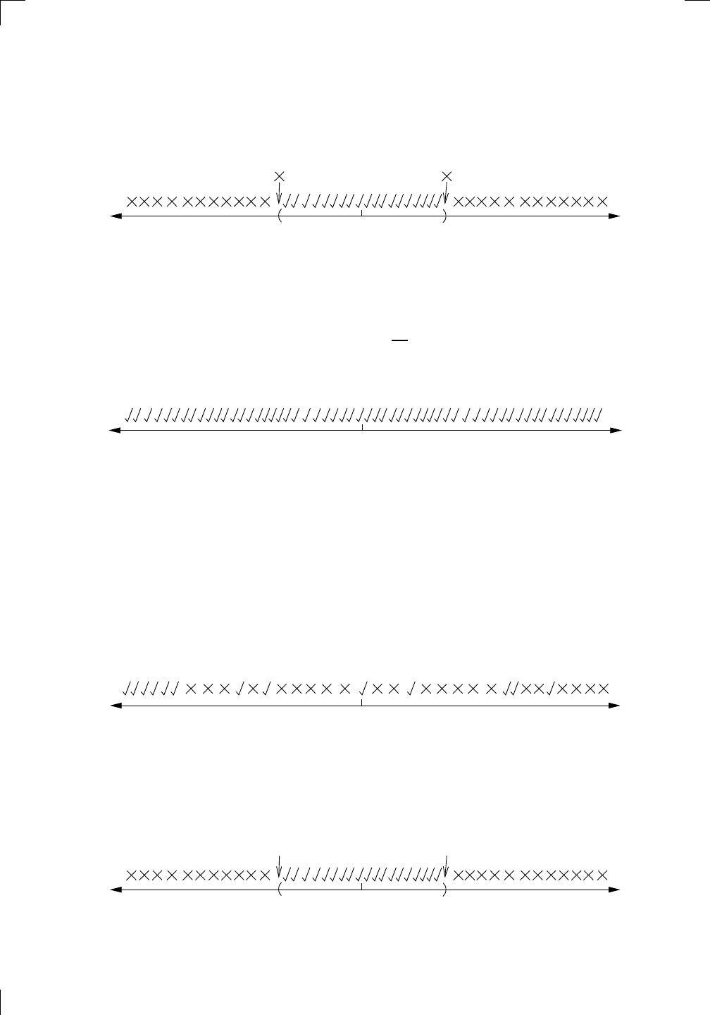
552 • Taylor and Power Series: How to Solve Problems
since the diagram would get crowded! We’ll just do enough to get the idea.)
For example, the geometric series
P
∞
n=0
x
n
converges when −1 < x < 1 and
diverges otherwise, so its picture looks like this:
PSfrag
replacements
(
a, b)
[
a, b]
(
a, b]
[
a, b)
(
a, ∞)
[
a, ∞)
(
−∞, b)
(
−∞, b]
(
−∞, ∞)
{
x : a < x < b}
{
x : a ≤ x ≤ b}
{
x : a < x ≤ b}
{
x : a ≤ x < b}
{
x : x ≥ a}
{
x : x > a}
{
x : x ≤ b}
{
x : x < b}
R
a
b
shado
w
0
1
4
−
2
3
−
3
g(
x) = x
2
f(
x) = x
3
g(
x) = x
2
f(
x) = x
3
mirror
(y = x)
f
−
1
(x) =
3
√
x
y = h
(x)
y = h
−
1
(x)
y =
(x − 1)
2
−
1
x
Same
height
−
x
Same
length,
opp
osite signs
y = −
2x
−
2
1
y =
1
2
x − 1
2
−
1
y =
2
x
y =
10
x
y =
2
−x
y =
log
2
(x)
4
3
units
mirror
(x-axis)
y = |
x|
y = |
log
2
(x)|
θ radians
θ units
30
◦
=
π
6
45
◦
=
π
4
60
◦
=
π
3
120
◦
=
2
π
3
135
◦
=
3
π
4
150
◦
=
5
π
6
90
◦
=
π
2
180
◦
= π
210
◦
=
7
π
6
225
◦
=
5
π
4
240
◦
=
4
π
3
270
◦
=
3
π
2
300
◦
=
5
π
3
315
◦
=
7
π
4
330
◦
=
11
π
6
0
◦
=
0 radians
θ
hypotenuse
opp
osite
adjacen
t
0
(≡ 2π)
π
2
π
3
π
2
I
I
I
I
II
IV
θ
(
x, y)
x
y
r
7
π
6
reference
angle
reference
angle =
π
6
sin
+
sin −
cos
+
cos −
tan
+
tan −
A
S
T
C
7
π
4
9
π
13
5
π
6
(this
angle is
5π
6
clo
ckwise)
1
2
1
2
3
4
5
6
0
−
1
−
2
−
3
−
4
−
5
−
6
−
3π
−
5
π
2
−
2π
−
3
π
2
−
π
−
π
2
3
π
3
π
5
π
2
2
π
3
π
2
π
π
2
y =
sin(x)
1
0
−
1
−
3π
−
5
π
2
−
2π
−
3
π
2
−
π
−
π
2
3
π
5
π
2
2
π
2
π
3
π
2
π
π
2
y =
sin(x)
y =
cos(x)
−
π
2
π
2
y =
tan(x), −
π
2
<
x <
π
2
0
−
π
2
π
2
y =
tan(x)
−
2π
−
3π
−
5
π
2
−
3
π
2
−
π
−
π
2
π
2
3
π
3
π
5
π
2
2
π
3
π
2
π
y =
sec(x)
y =
csc(x)
y =
cot(x)
y = f (
x)
−
1
1
2
y = g(
x)
3
y = h
(x)
4
5
−
2
f(
x) =
1
x
g(
x) =
1
x
2
etc.
0
1
π
1
2
π
1
3
π
1
4
π
1
5
π
1
6
π
1
7
π
g(
x) = sin
1
x
1
0
−
1
L
10
100
200
y =
π
2
y = −
π
2
y =
tan
−1
(x)
π
2
π
y =
sin(
x)
x
,
x > 3
0
1
−
1
a
L
f(
x) = x sin (1/x)
(0 <
x < 0.3)
h
(x) = x
g(
x) = −x
a
L
lim
x
→a
+
f(x) = L
lim
x
→a
+
f(x) = ∞
lim
x
→a
+
f(x) = −∞
lim
x
→a
+
f(x) DNE
lim
x
→a
−
f(x) = L
lim
x
→a
−
f(x) = ∞
lim
x
→a
−
f(x) = −∞
lim
x
→a
−
f(x) DNE
M
}
lim
x
→a
−
f(x) = M
lim
x
→a
f(x) = L
lim
x
→a
f(x) DNE
lim
x
→∞
f(x) = L
lim
x
→∞
f(x) = ∞
lim
x
→∞
f(x) = −∞
lim
x
→∞
f(x) DNE
lim
x
→−∞
f(x) = L
lim
x
→−∞
f(x) = ∞
lim
x
→−∞
f(x) = −∞
lim
x
→−∞
f(x) DNE
lim
x →a
+
f(
x) = ∞
lim
x →a
+
f(
x) = −∞
lim
x →a
−
f(
x) = ∞
lim
x →a
−
f(
x) = −∞
lim
x →a
f(
x) = ∞
lim
x →a
f(
x) = −∞
lim
x →a
f(
x) DNE
y = f (
x)
a
y =
|
x|
x
1
−
1
y =
|
x + 2|
x +
2
1
−
1
−
2
1
2
3
4
a
a
b
y = x sin
1
x
y = x
y = −
x
a
b
c
d
C
a
b
c
d
−
1
0
1
2
3
time
y
t
u
(
t, f(t))
(
u, f(u))
time
y
t
u
y
x
(
x, f(x))
y = |
x|
(
z, f(z))
z
y = f (
x)
a
tangen
t at x = a
b
tangen
t at x = b
c
tangen
t at x = c
y = x
2
tangen
t
at x = −
1
u
v
uv
u +
∆u
v +
∆v
(
u + ∆u)(v + ∆v)
∆
u
∆
v
u
∆v
v∆
u
∆
u∆v
y = f (
x)
1
2
−
2
y = |
x
2
− 4|
y = x
2
− 4
y = −
2x + 5
y = g(
x)
1
2
3
4
5
6
7
8
9
0
−
1
−
2
−
3
−
4
−
5
−
6
y = f (
x)
3
−
3
3
−
3
0
−
1
2
easy
hard
flat
y = f
0
(
x)
3
−
3
0
−
1
2
1
−
1
y =
sin(x)
y = x
x
A
B
O
1
C
D
sin(
x)
tan(
x)
y =
sin
(x)
x
π
2
π
1
−
1
x =
0
a =
0
x
> 0
a
> 0
x
< 0
a
< 0
rest
position
+
−
y = x
2
sin
1
x
N
A
B
H
a
b
c
O
H
A
B
C
D
h
r
R
θ
1000
2000
α
β
p
h
y = g(
x) = log
b
(x)
y = f(
x) = b
x
y = e
x
5
10
1
2
3
4
0
−
1
−
2
−
3
−
4
y =
ln(x)
y =
cosh(x)
y =
sinh(x)
y =
tanh(x)
y =
sech(x)
y =
csch(x)
y =
coth(x)
1
−
1
y = f (
x)
original
function
in
verse function
slop
e = 0 at (x, y)
slop
e is infinite at (y, x)
−
108
2
5
1
2
1
2
3
4
5
6
0
−
1
−
2
−
3
−
4
−
5
−
6
−
3π
−
5
π
2
−
2π
−
3
π
2
−
π
−
π
2
3
π
3
π
5
π
2
2
π
3
π
2
π
π
2
y =
sin(x)
1
0
−
1
−
3π
−
5
π
2
−
2π
−
3
π
2
−
π
−
π
2
3
π
5
π
2
2
π
2
π
3
π
2
π
π
2
y =
sin(x)
y =
sin(x), −
π
2
≤ x ≤
π
2
−
2
−
1
0
2
π
2
−
π
2
y =
sin
−1
(x)
y =
cos(x)
π
π
2
y =
cos
−1
(x)
−
π
2
1
x
α
β
y =
tan(x)
y =
tan(x)
1
y =
tan
−1
(x)
y =
sec(x)
y =
sec
−1
(x)
y =
csc
−1
(x)
y =
cot
−1
(x)
1
y =
cosh
−1
(x)
y =
sinh
−1
(x)
y =
tanh
−1
(x)
y =
sech
−1
(x)
y =
csch
−1
(x)
y =
coth
−1
(x)
(0
, 3)
(2
, −1)
(5
, 2)
(7
, 0)
(
−1, 44)
(0
, 1)
(1
, −12)
(2
, 305)
y =
1
2
(2
, 3)
y = f (
x)
y = g(
x)
a
b
c
a
b
c
s
c
0
c
1
(
a, f(a))
(
b, f(b))
1
2
1
2
3
4
5
6
0
−
1
−
2
−
3
−
4
−
5
−
6
−
3π
−
5
π
2
−
2π
−
3
π
2
−
π
−
π
2
3
π
3
π
5
π
2
2
π
3
π
2
π
π
2
y =
sin(x)
1
0
−
1
−
3π
−
5
π
2
−
2π
−
3
π
2
−
π
−
π
2
3
π
5
π
2
2
π
2
π
3
π
2
π
π
2
c
OR
Lo
cal maximum
Lo
cal minimum
Horizon
tal point of inflection
1
e
y = f
0
(
x)
y = f(
x) = x ln(x)
−
1
e
?
y = f(
x) = x
3
y = g(
x) = x
4
x
f(
x)
−
3
−
2
−
1
0
1
2
1
2
3
4
+
−
?
1
5
6
3
f
0
(
x)
2 −
1
2
√
6
2
+
1
2
√
6
f
00
(
x)
7
8
g
00
(
x)
f
00
(
x)
0
y =
(
x − 3)(x − 1)
2
x
3
(
x + 2)
y = x ln
(x)
1
e
−
1
e
5
−
108
2
α
β
2 −
1
2
√
6
2
+
1
2
√
6
y = x
2
(
x − 5)
3
−
e
−
1/2
√
3
e
−
1/2
√
3
−
e
−3/2
e
−
3/2
−
1
√
3
1
√
3
−
1
1
y = xe
−
3x
2
/2
y =
x
3
− 6
x
2
+ 13x − 8
x
28
2
600
500
400
300
200
100
0
−
100
−
200
−
300
−
400
−
500
−
600
0
10
−
10
5
−
5
20
−
20
15
−
15
0
4
5
6
x
P
0
(
x)
+
−
−
existing
fence
new
fence
enclosure
A
h
b
H
99
100
101
h
dA/dh
r
h
1
2
7
shallo
w
deep
LAND
SEA
N
y
z
s
t
3
11
9
L
(11)
√
11
y = L
(x)
y = f (
x)
11
y = L
(x)
y = f (
x)
F
P
a
a +
∆x
f(
a + ∆x)
L
(a + ∆x)
f(
a)
error
d
f
∆
x
a
b
y = f (
x)
true
zero
starting
approximation
b
etter approximation
v
t
3
5
50
40
60
4
20
30
25
t
1
t
2
t
3
t
4
t
n
−2
t
n
−1
t
0
= a
t
n
= b
v
1
v
2
v
3
v
4
v
n
−1
v
n
−
30
6
30
|
v|
a
b
p
q
c
v(
c)
v(
c
1
)
v(
c
2
)
v(
c
3
)
v(
c
4
)
v(
c
5
)
v(
c
6
)
t
1
t
2
t
3
t
4
t
5
c
1
c
2
c
3
c
4
c
5
c
6
t
0
=
a
t
6
=
b
t
16
=
b
t
10
=
b
a
b
x
y
y = f (
x)
1
2
y = x
5
0
−
2
y =
1
a
b
y =
sin(x)
π
−
π
0
−
1
−
2
0
2
4
y = x
2
0
1
2
3
4
2
n
4
n
6
n
2(
n−2)
n
2(
n−1)
n
2
n
n
=
2
width
of each interval =
2
n
−
2
1
3
0
I
I
I
I
II
IV
4
y
dx
y = −
x
2
− 2x + 3
3
−
5
y = |−
x
2
− 2x + 3|
I
I
I
I
Ia
5
3
0
1
2
a
b
y = f (
x)
y = g(
x)
y = x
2
a
b
5
3
0
1
2
y =
√
x
2
√
2
2
2
dy
x
2
a
b
y = f (
x)
y = g(
x)
M
m
1
2
−
1
−
2
0
y = e
−
x
2
1
2
e
−
1/4
f
a
v
y = f
a
v
c
A
M
0
1
2
a
b
x
t
y = f(
t)
F (
x )
y = f(
t)
F (
x + h )
x + h
F (
x + h) − F (x)
f(
x)
1
2
y =
sin(x)
π
−
π
−
1
−
2
y =
1
x
y = x
2
1
2
1
−
1
y =
ln|x|
θ
a
x
a
x
p
a
2
− x
2
3
x
p
9 − x
2
p
x
2
+ a
2
x
a
p
x
2
+ 15
x
√
15
x
p
x
2
− a
2
a
x
p
x
2
− 4
2
x
−
p
x
2
− a
2
a
x
−
p
x
2
− 4
2
y = f (x)
a
b
a + ε
ε
Z
b
a+ε
f(x) dx
small
even smaller
y = g(x)
infinite area
finite area
1
y =
1
x
y =
1
x
p
, p < 1 (typical)
y =
1
x
p
, p > 1 (typical)
a
1
a
2
a
3
a
4
a
5
a
6
a
7
a
8
1
2
3
4
5
6
7
8
n
a
n
x
y
y = f (x)
(a, f(a))
a
−1
0
1
Note that I took special care to indicate the divergence at the endpoints 1
and −1.
On the other hand, we’ve seen that the series
∞
X
n=0
x
n
n!
converges for all x (to e
x
, of course), so its picture looks like this:
PSfrag
replacements
(
a, b)
[
a, b]
(
a, b]
[
a, b)
(
a, ∞)
[
a, ∞)
(
−∞, b)
(
−∞, b]
(
−∞, ∞)
{
x : a < x < b}
{
x : a ≤ x ≤ b}
{
x : a < x ≤ b}
{
x : a ≤ x < b}
{
x : x ≥ a}
{
x : x > a}
{
x : x ≤ b}
{
x : x < b}
R
a
b
shado
w
0
1
4
−
2
3
−
3
g(
x) = x
2
f(
x) = x
3
g(
x) = x
2
f(
x) = x
3
mirror
(y = x)
f
−
1
(x) =
3
√
x
y = h
(x)
y = h
−
1
(x)
y =
(x − 1)
2
−
1
x
Same
height
−
x
Same
length,
opp
osite signs
y = −
2x
−
2
1
y =
1
2
x − 1
2
−
1
y =
2
x
y =
10
x
y =
2
−x
y =
log
2
(x)
4
3
units
mirror
(x-axis)
y = |
x|
y = |
log
2
(x)|
θ radians
θ units
30
◦
=
π
6
45
◦
=
π
4
60
◦
=
π
3
120
◦
=
2
π
3
135
◦
=
3
π
4
150
◦
=
5
π
6
90
◦
=
π
2
180
◦
= π
210
◦
=
7
π
6
225
◦
=
5
π
4
240
◦
=
4
π
3
270
◦
=
3
π
2
300
◦
=
5
π
3
315
◦
=
7
π
4
330
◦
=
11
π
6
0
◦
=
0 radians
θ
hypotenuse
opp
osite
adjacen
t
0
(≡ 2π)
π
2
π
3
π
2
I
I
I
I
II
IV
θ
(
x, y)
x
y
r
7
π
6
reference
angle
reference
angle =
π
6
sin
+
sin −
cos
+
cos −
tan
+
tan −
A
S
T
C
7
π
4
9
π
13
5
π
6
(this
angle is
5π
6
clo
ckwise)
1
2
1
2
3
4
5
6
0
−
1
−
2
−
3
−
4
−
5
−
6
−
3π
−
5
π
2
−
2π
−
3
π
2
−
π
−
π
2
3
π
3
π
5
π
2
2
π
3
π
2
π
π
2
y =
sin(x)
1
0
−
1
−
3π
−
5
π
2
−
2π
−
3
π
2
−
π
−
π
2
3
π
5
π
2
2
π
2
π
3
π
2
π
π
2
y =
sin(x)
y =
cos(x)
−
π
2
π
2
y =
tan(x), −
π
2
<
x <
π
2
0
−
π
2
π
2
y =
tan(x)
−
2π
−
3π
−
5
π
2
−
3
π
2
−
π
−
π
2
π
2
3
π
3
π
5
π
2
2
π
3
π
2
π
y =
sec(x)
y =
csc(x)
y =
cot(x)
y = f (
x)
−
1
1
2
y = g(
x)
3
y = h
(x)
4
5
−
2
f(
x) =
1
x
g(
x) =
1
x
2
etc.
0
1
π
1
2
π
1
3
π
1
4
π
1
5
π
1
6
π
1
7
π
g(
x) = sin
1
x
1
0
−
1
L
10
100
200
y =
π
2
y = −
π
2
y =
tan
−1
(x)
π
2
π
y =
sin(
x)
x
,
x > 3
0
1
−
1
a
L
f(
x) = x sin (1/x)
(0 <
x < 0.3)
h
(x) = x
g(
x) = −x
a
L
lim
x
→a
+
f(x) = L
lim
x
→a
+
f(x) = ∞
lim
x
→a
+
f(x) = −∞
lim
x
→a
+
f(x) DNE
lim
x
→a
−
f(x) = L
lim
x
→a
−
f(x) = ∞
lim
x
→a
−
f(x) = −∞
lim
x
→a
−
f(x) DNE
M
}
lim
x
→a
−
f(x) = M
lim
x
→a
f(x) = L
lim
x
→a
f(x) DNE
lim
x
→∞
f(x) = L
lim
x
→∞
f(x) = ∞
lim
x
→∞
f(x) = −∞
lim
x
→∞
f(x) DNE
lim
x
→−∞
f(x) = L
lim
x
→−∞
f(x) = ∞
lim
x
→−∞
f(x) = −∞
lim
x
→−∞
f(x) DNE
lim
x →a
+
f(
x) = ∞
lim
x →a
+
f(
x) = −∞
lim
x →a
−
f(
x) = ∞
lim
x →a
−
f(
x) = −∞
lim
x →a
f(
x) = ∞
lim
x →a
f(
x) = −∞
lim
x →a
f(
x) DNE
y = f (
x)
a
y =
|
x|
x
1
−
1
y =
|
x + 2|
x +
2
1
−
1
−
2
1
2
3
4
a
a
b
y = x sin
1
x
y = x
y = −
x
a
b
c
d
C
a
b
c
d
−
1
0
1
2
3
time
y
t
u
(
t, f(t))
(
u, f(u))
time
y
t
u
y
x
(
x, f(x))
y = |
x|
(
z, f(z))
z
y = f (
x)
a
tangen
t at x = a
b
tangen
t at x = b
c
tangen
t at x = c
y = x
2
tangen
t
at x = −
1
u
v
uv
u +
∆u
v +
∆v
(
u + ∆u)(v + ∆v)
∆
u
∆
v
u
∆v
v∆
u
∆
u∆v
y = f (
x)
1
2
−
2
y = |
x
2
− 4|
y = x
2
− 4
y = −
2x + 5
y = g(
x)
1
2
3
4
5
6
7
8
9
0
−
1
−
2
−
3
−
4
−
5
−
6
y = f (
x)
3
−
3
3
−
3
0
−
1
2
easy
hard
flat
y = f
0
(
x)
3
−
3
0
−
1
2
1
−
1
y =
sin(x)
y = x
x
A
B
O
1
C
D
sin(
x)
tan(
x)
y =
sin
(x)
x
π
2
π
1
−
1
x =
0
a =
0
x
> 0
a
> 0
x
< 0
a
< 0
rest
position
+
−
y = x
2
sin
1
x
N
A
B
H
a
b
c
O
H
A
B
C
D
h
r
R
θ
1000
2000
α
β
p
h
y = g(
x) = log
b
(x)
y = f(
x) = b
x
y = e
x
5
10
1
2
3
4
0
−
1
−
2
−
3
−
4
y =
ln(x)
y =
cosh(x)
y =
sinh(x)
y =
tanh(x)
y =
sech(x)
y =
csch(x)
y =
coth(x)
1
−
1
y = f (
x)
original
function
in
verse function
slop
e = 0 at (x, y)
slop
e is infinite at (y, x)
−
108
2
5
1
2
1
2
3
4
5
6
0
−
1
−
2
−
3
−
4
−
5
−
6
−
3π
−
5
π
2
−
2π
−
3
π
2
−
π
−
π
2
3
π
3
π
5
π
2
2
π
3
π
2
π
π
2
y =
sin(x)
1
0
−
1
−
3π
−
5
π
2
−
2π
−
3
π
2
−
π
−
π
2
3
π
5
π
2
2
π
2
π
3
π
2
π
π
2
y =
sin(x)
y =
sin(x), −
π
2
≤ x ≤
π
2
−
2
−
1
0
2
π
2
−
π
2
y =
sin
−1
(x)
y =
cos(x)
π
π
2
y =
cos
−1
(x)
−
π
2
1
x
α
β
y =
tan(x)
y =
tan(x)
1
y =
tan
−1
(x)
y =
sec(x)
y =
sec
−1
(x)
y =
csc
−1
(x)
y =
cot
−1
(x)
1
y =
cosh
−1
(x)
y =
sinh
−1
(x)
y =
tanh
−1
(x)
y =
sech
−1
(x)
y =
csch
−1
(x)
y =
coth
−1
(x)
(0
, 3)
(2
, −1)
(5
, 2)
(7
, 0)
(
−1, 44)
(0
, 1)
(1
, −12)
(2
, 305)
y =
1
2
(2
, 3)
y = f (
x)
y = g(
x)
a
b
c
a
b
c
s
c
0
c
1
(
a, f(a))
(
b, f(b))
1
2
1
2
3
4
5
6
0
−
1
−
2
−
3
−
4
−
5
−
6
−
3π
−
5
π
2
−
2π
−
3
π
2
−
π
−
π
2
3
π
3
π
5
π
2
2
π
3
π
2
π
π
2
y =
sin(x)
1
0
−
1
−
3π
−
5
π
2
−
2π
−
3
π
2
−
π
−
π
2
3
π
5
π
2
2
π
2
π
3
π
2
π
π
2
c
OR
Lo
cal maximum
Lo
cal minimum
Horizon
tal point of inflection
1
e
y = f
0
(
x)
y = f(
x) = x ln(x)
−
1
e
?
y = f(
x) = x
3
y = g(
x) = x
4
x
f(
x)
−
3
−
2
−
1
0
1
2
1
2
3
4
+
−
?
1
5
6
3
f
0
(
x)
2 −
1
2
√
6
2
+
1
2
√
6
f
00
(
x)
7
8
g
00
(
x)
f
00
(
x)
0
y =
(
x − 3)(x − 1)
2
x
3
(
x + 2)
y = x ln
(x)
1
e
−
1
e
5
−
108
2
α
β
2 −
1
2
√
6
2
+
1
2
√
6
y = x
2
(
x − 5)
3
−
e
−
1/2
√
3
e
−
1/2
√
3
−
e
−3/2
e
−
3/2
−
1
√
3
1
√
3
−
1
1
y = xe
−
3x
2
/2
y =
x
3
− 6
x
2
+ 13x − 8
x
28
2
600
500
400
300
200
100
0
−
100
−
200
−
300
−
400
−
500
−
600
0
10
−
10
5
−
5
20
−
20
15
−
15
0
4
5
6
x
P
0
(
x)
+
−
−
existing
fence
new
fence
enclosure
A
h
b
H
99
100
101
h
dA/dh
r
h
1
2
7
shallo
w
deep
LAND
SEA
N
y
z
s
t
3
11
9
L
(11)
√
11
y = L
(x)
y = f (
x)
11
y = L
(x)
y = f (
x)
F
P
a
a +
∆x
f(
a + ∆x)
L
(a + ∆x)
f(
a)
error
d
f
∆
x
a
b
y = f (
x)
true
zero
starting
approximation
b
etter approximation
v
t
3
5
50
40
60
4
20
30
25
t
1
t
2
t
3
t
4
t
n
−2
t
n
−1
t
0
= a
t
n
= b
v
1
v
2
v
3
v
4
v
n
−1
v
n
−
30
6
30
|
v|
a
b
p
q
c
v(
c)
v(
c
1
)
v(
c
2
)
v(
c
3
)
v(
c
4
)
v(
c
5
)
v(
c
6
)
t
1
t
2
t
3
t
4
t
5
c
1
c
2
c
3
c
4
c
5
c
6
t
0
=
a
t
6
=
b
t
16
=
b
t
10
=
b
a
b
x
y
y = f (
x)
1
2
y = x
5
0
−
2
y =
1
a
b
y =
sin(x)
π
−
π
0
−
1
−
2
0
2
4
y = x
2
0
1
2
3
4
2
n
4
n
6
n
2(
n−2)
n
2(
n−1)
n
2
n
n
=
2
width
of each interval =
2
n
−
2
1
3
0
I
I
I
I
II
IV
4
y
dx
y = −
x
2
− 2x + 3
3
−
5
y = |−
x
2
− 2x + 3|
I
I
I
I
Ia
5
3
0
1
2
a
b
y = f (
x)
y = g(
x)
y = x
2
a
b
5
3
0
1
2
y =
√
x
2
√
2
2
2
dy
x
2
a
b
y = f (
x)
y = g(
x)
M
m
1
2
−
1
−
2
0
y = e
−
x
2
1
2
e
−
1/4
f
a
v
y = f
a
v
c
A
M
0
1
2
a
b
x
t
y = f(
t)
F (
x )
y = f(
t)
F (
x + h )
x + h
F (
x + h) − F (x)
f(
x)
1
2
y =
sin(x)
π
−
π
−
1
−
2
y =
1
x
y = x
2
1
2
1
−
1
y =
ln|x|
θ
a
x
a
x
p
a
2
− x
2
3
x
p
9 − x
2
p
x
2
+ a
2
x
a
p
x
2
+ 15
x
√
15
x
p
x
2
− a
2
a
x
p
x
2
− 4
2
x
−
p
x
2
− a
2
a
x
−
p
x
2
− 4
2
y = f (x)
a
b
a + ε
ε
Z
b
a+ε
f(x) dx
small
even smaller
y = g(x)
infinite area
finite area
1
y =
1
x
y =
1
x
p
, p < 1 (typical)
y =
1
x
p
, p > 1 (typical)
a
1
a
2
a
3
a
4
a
5
a
6
a
7
a
8
1
2
3
4
5
6
7
8
n
a
n
x
y
y = f (x)
(a, f(a))
a
−1
0
1
It seems like this could be pretty unpredictable. One thing that we can say
for sure is that the power series always converges at x = a. In fact, if you
substitute x = a into
∞
X
n=0
a
n
(x − a)
n
= a
0
+ a
1
(x − a) + a
2
(x − a)
2
+ ··· ,
you can see that all the terms vanish except a
0
. So, the series evidently
converges (to a
0
). Unfortunately, the value x = a is the only value for which
we can predict the convergence for certain. How about the other values?
Maybe it would be possible to get a hodgepodge of checks and crosses, like
this:
PSfrag
replacements
(
a, b)
[
a, b]
(
a, b]
[
a, b)
(
a, ∞)
[
a, ∞)
(
−∞, b)
(
−∞, b]
(
−∞, ∞)
{
x : a < x < b}
{
x : a ≤ x ≤ b}
{
x : a < x ≤ b}
{
x : a ≤ x < b}
{
x : x ≥ a}
{
x : x > a}
{
x : x ≤ b}
{
x : x < b}
R
a
b
shado
w
0
1
4
−
2
3
−
3
g(
x) = x
2
f(
x) = x
3
g(
x) = x
2
f(
x) = x
3
mirror
(y = x)
f
−
1
(x) =
3
√
x
y = h
(x)
y = h
−
1
(x)
y =
(x − 1)
2
−
1
x
Same
height
−
x
Same
length,
opp
osite signs
y = −
2x
−
2
1
y =
1
2
x − 1
2
−
1
y =
2
x
y =
10
x
y =
2
−x
y =
log
2
(x)
4
3
units
mirror
(x-axis)
y = |
x|
y = |
log
2
(x)|
θ radians
θ units
30
◦
=
π
6
45
◦
=
π
4
60
◦
=
π
3
120
◦
=
2
π
3
135
◦
=
3
π
4
150
◦
=
5
π
6
90
◦
=
π
2
180
◦
= π
210
◦
=
7
π
6
225
◦
=
5
π
4
240
◦
=
4
π
3
270
◦
=
3
π
2
300
◦
=
5
π
3
315
◦
=
7
π
4
330
◦
=
11
π
6
0
◦
=
0 radians
θ
hypotenuse
opp
osite
adjacen
t
0
(≡ 2π)
π
2
π
3
π
2
I
I
I
I
II
IV
θ
(
x, y)
x
y
r
7
π
6
reference
angle
reference
angle =
π
6
sin
+
sin −
cos
+
cos −
tan
+
tan −
A
S
T
C
7
π
4
9
π
13
5
π
6
(this
angle is
5π
6
clo
ckwise)
1
2
1
2
3
4
5
6
0
−
1
−
2
−
3
−
4
−
5
−
6
−
3π
−
5
π
2
−
2π
−
3
π
2
−
π
−
π
2
3
π
3
π
5
π
2
2
π
3
π
2
π
π
2
y =
sin(x)
1
0
−
1
−
3π
−
5
π
2
−
2π
−
3
π
2
−
π
−
π
2
3
π
5
π
2
2
π
2
π
3
π
2
π
π
2
y =
sin(x)
y =
cos(x)
−
π
2
π
2
y =
tan(x), −
π
2
<
x <
π
2
0
−
π
2
π
2
y =
tan(x)
−
2π
−
3π
−
5
π
2
−
3
π
2
−
π
−
π
2
π
2
3
π
3
π
5
π
2
2
π
3
π
2
π
y =
sec(x)
y =
csc(x)
y =
cot(x)
y = f (
x)
−
1
1
2
y = g(
x)
3
y = h
(x)
4
5
−
2
f(
x) =
1
x
g(
x) =
1
x
2
etc.
0
1
π
1
2
π
1
3
π
1
4
π
1
5
π
1
6
π
1
7
π
g(
x) = sin
1
x
1
0
−
1
L
10
100
200
y =
π
2
y = −
π
2
y =
tan
−1
(x)
π
2
π
y =
sin(
x)
x
,
x > 3
0
1
−
1
a
L
f(
x) = x sin (1/x)
(0 <
x < 0.3)
h
(x) = x
g(
x) = −x
a
L
lim
x
→a
+
f(x) = L
lim
x
→a
+
f(x) = ∞
lim
x
→a
+
f(x) = −∞
lim
x
→a
+
f(x) DNE
lim
x
→a
−
f(x) = L
lim
x
→a
−
f(x) = ∞
lim
x
→a
−
f(x) = −∞
lim
x
→a
−
f(x) DNE
M
}
lim
x
→a
−
f(x) = M
lim
x
→a
f(x) = L
lim
x
→a
f(x) DNE
lim
x
→∞
f(x) = L
lim
x
→∞
f(x) = ∞
lim
x
→∞
f(x) = −∞
lim
x
→∞
f(x) DNE
lim
x
→−∞
f(x) = L
lim
x
→−∞
f(x) = ∞
lim
x
→−∞
f(x) = −∞
lim
x
→−∞
f(x) DNE
lim
x →a
+
f(
x) = ∞
lim
x →a
+
f(
x) = −∞
lim
x →a
−
f(
x) = ∞
lim
x →a
−
f(
x) = −∞
lim
x →a
f(
x) = ∞
lim
x →a
f(
x) = −∞
lim
x →a
f(
x) DNE
y = f (
x)
a
y =
|
x|
x
1
−
1
y =
|
x + 2|
x +
2
1
−
1
−
2
1
2
3
4
a
a
b
y = x sin
1
x
y = x
y = −
x
a
b
c
d
C
a
b
c
d
−
1
0
1
2
3
time
y
t
u
(
t, f(t))
(
u, f(u))
time
y
t
u
y
x
(
x, f(x))
y = |
x|
(
z, f(z))
z
y = f (
x)
a
tangen
t at x = a
b
tangen
t at x = b
c
tangen
t at x = c
y = x
2
tangen
t
at x = −
1
u
v
uv
u +
∆u
v +
∆v
(
u + ∆u)(v + ∆v)
∆
u
∆
v
u
∆v
v∆
u
∆
u∆v
y = f (
x)
1
2
−
2
y = |
x
2
− 4|
y = x
2
− 4
y = −
2x + 5
y = g(
x)
1
2
3
4
5
6
7
8
9
0
−
1
−
2
−
3
−
4
−
5
−
6
y = f (
x)
3
−
3
3
−
3
0
−
1
2
easy
hard
flat
y = f
0
(
x)
3
−
3
0
−
1
2
1
−
1
y =
sin(x)
y = x
x
A
B
O
1
C
D
sin(
x)
tan(
x)
y =
sin
(x)
x
π
2
π
1
−
1
x =
0
a =
0
x
> 0
a
> 0
x
< 0
a
< 0
rest
position
+
−
y = x
2
sin
1
x
N
A
B
H
a
b
c
O
H
A
B
C
D
h
r
R
θ
1000
2000
α
β
p
h
y = g(
x) = log
b
(x)
y = f(
x) = b
x
y = e
x
5
10
1
2
3
4
0
−
1
−
2
−
3
−
4
y =
ln(x)
y =
cosh(x)
y =
sinh(x)
y =
tanh(x)
y =
sech(x)
y =
csch(x)
y =
coth(x)
1
−
1
y = f (
x)
original
function
in
verse function
slop
e = 0 at (x, y)
slop
e is infinite at (y, x)
−
108
2
5
1
2
1
2
3
4
5
6
0
−
1
−
2
−
3
−
4
−
5
−
6
−
3π
−
5
π
2
−
2π
−
3
π
2
−
π
−
π
2
3
π
3
π
5
π
2
2
π
3
π
2
π
π
2
y =
sin(x)
1
0
−
1
−
3π
−
5
π
2
−
2π
−
3
π
2
−
π
−
π
2
3
π
5
π
2
2
π
2
π
3
π
2
π
π
2
y =
sin(x)
y =
sin(x), −
π
2
≤ x ≤
π
2
−
2
−
1
0
2
π
2
−
π
2
y =
sin
−1
(x)
y =
cos(x)
π
π
2
y =
cos
−1
(x)
−
π
2
1
x
α
β
y =
tan(x)
y =
tan(x)
1
y =
tan
−1
(x)
y =
sec(x)
y =
sec
−1
(x)
y =
csc
−1
(x)
y =
cot
−1
(x)
1
y =
cosh
−1
(x)
y =
sinh
−1
(x)
y =
tanh
−1
(x)
y =
sech
−1
(x)
y =
csch
−1
(x)
y =
coth
−1
(x)
(0
, 3)
(2
, −1)
(5
, 2)
(7
, 0)
(
−1, 44)
(0
, 1)
(1
, −12)
(2
, 305)
y =
1
2
(2
, 3)
y = f (
x)
y = g(
x)
a
b
c
a
b
c
s
c
0
c
1
(
a, f(a))
(
b, f(b))
1
2
1
2
3
4
5
6
0
−
1
−
2
−
3
−
4
−
5
−
6
−
3π
−
5
π
2
−
2π
−
3
π
2
−
π
−
π
2
3
π
3
π
5
π
2
2
π
3
π
2
π
π
2
y =
sin(x)
1
0
−
1
−
3π
−
5
π
2
−
2π
−
3
π
2
−
π
−
π
2
3
π
5
π
2
2
π
2
π
3
π
2
π
π
2
c
OR
Lo
cal maximum
Lo
cal minimum
Horizon
tal point of inflection
1
e
y = f
0
(
x)
y = f(
x) = x ln(x)
−
1
e
?
y = f(
x) = x
3
y = g(
x) = x
4
x
f(
x)
−
3
−
2
−
1
0
1
2
1
2
3
4
+
−
?
1
5
6
3
f
0
(
x)
2 −
1
2
√
6
2
+
1
2
√
6
f
00
(
x)
7
8
g
00
(
x)
f
00
(
x)
0
y =
(
x − 3)(x − 1)
2
x
3
(
x + 2)
y = x ln
(x)
1
e
−
1
e
5
−
108
2
α
β
2 −
1
2
√
6
2
+
1
2
√
6
y = x
2
(
x − 5)
3
−
e
−
1/2
√
3
e
−
1/2
√
3
−
e
−3/2
e
−
3/2
−
1
√
3
1
√
3
−
1
1
y = xe
−
3x
2
/2
y =
x
3
− 6
x
2
+ 13x − 8
x
28
2
600
500
400
300
200
100
0
−
100
−
200
−
300
−
400
−
500
−
600
0
10
−
10
5
−
5
20
−
20
15
−
15
0
4
5
6
x
P
0
(
x)
+
−
−
existing
fence
new
fence
enclosure
A
h
b
H
99
100
101
h
dA/dh
r
h
1
2
7
shallo
w
deep
LAND
SEA
N
y
z
s
t
3
11
9
L
(11)
√
11
y = L
(x)
y = f (
x)
11
y = L
(x)
y = f (
x)
F
P
a
a +
∆x
f(
a + ∆x)
L
(a + ∆x)
f(
a)
error
d
f
∆
x
a
b
y = f (
x)
true
zero
starting
approximation
b
etter approximation
v
t
3
5
50
40
60
4
20
30
25
t
1
t
2
t
3
t
4
t
n
−2
t
n
−1
t
0
= a
t
n
= b
v
1
v
2
v
3
v
4
v
n
−1
v
n
−
30
6
30
|
v|
a
b
p
q
c
v(
c)
v(
c
1
)
v(
c
2
)
v(
c
3
)
v(
c
4
)
v(
c
5
)
v(
c
6
)
t
1
t
2
t
3
t
4
t
5
c
1
c
2
c
3
c
4
c
5
c
6
t
0
=
a
t
6
=
b
t
16
=
b
t
10
=
b
a
b
x
y
y = f (
x)
1
2
y = x
5
0
−
2
y =
1
a
b
y =
sin(x)
π
−
π
0
−
1
−
2
0
2
4
y = x
2
0
1
2
3
4
2
n
4
n
6
n
2(
n−2)
n
2(
n−1)
n
2
n
n
=
2
width
of each interval =
2
n
−
2
1
3
0
I
I
I
I
II
IV
4
y
dx
y = −
x
2
− 2x + 3
3
−
5
y = |−
x
2
− 2x + 3|
I
I
I
I
Ia
5
3
0
1
2
a
b
y = f (
x)
y = g(
x)
y = x
2
a
b
5
3
0
1
2
y =
√
x
2
√
2
2
2
dy
x
2
a
b
y = f (
x)
y = g(
x)
M
m
1
2
−
1
−
2
0
y = e
−
x
2
1
2
e
−
1/4
f
a
v
y = f
a
v
c
A
M
0
1
2
a
b
x
t
y = f(
t)
F (
x )
y = f(
t)
F (
x + h )
x + h
F (
x + h) − F (x)
f(
x)
1
2
y =
sin(x)
π
−
π
−
1
−
2
y =
1
x
y = x
2
1
2
1
−1
y = ln|x|
θ
a
x
a
x
p
a
2
− x
2
3
x
p
9 − x
2
p
x
2
+ a
2
x
a
p
x
2
+ 15
x
√
15
x
p
x
2
− a
2
a
x
p
x
2
− 4
2
x
−
p
x
2
− a
2
a
x
−
p
x
2
− 4
2
y = f (x)
a
b
a + ε
ε
Z
b
a+ε
f(x) dx
small
even smaller
y = g(x)
infinite area
finite area
1
y =
1
x
y =
1
x
p
, p < 1 (typical)
y =
1
x
p
, p > 1 (typical)
a
1
a
2
a
3
a
4
a
5
a
6
a
7
a
8
1
2
3
4
5
6
7
8
n
a
n
x
y
y = f (x)
(a, f(a))
a
−1
0
1
a
It turns out that the above picture can’t happen for power series. Specifically,
there are only three possibilities that can occur:
1. There is some number R > 0, called the radius of convergence of the
power series, such that the picture looks like this:
PSfrag
replacements
(
a, b)
[
a, b]
(
a, b]
[
a, b)
(
a, ∞)
[
a, ∞)
(
−∞, b)
(
−∞, b]
(
−∞, ∞)
{
x : a < x < b}
{
x : a ≤ x ≤ b}
{
x : a < x ≤ b}
{
x : a ≤ x < b}
{
x : x ≥ a}
{
x : x > a}
{
x : x ≤ b}
{
x : x < b}
R
a
b
shado
w
0
1
4
−
2
3
−
3
g(
x) = x
2
f(
x) = x
3
g(
x) = x
2
f(
x) = x
3
mirror
(y = x)
f
−
1
(x) =
3
√
x
y = h
(x)
y = h
−
1
(x)
y =
(x − 1)
2
−
1
x
Same
height
−
x
Same
length,
opp
osite signs
y = −
2x
−
2
1
y =
1
2
x − 1
2
−
1
y =
2
x
y =
10
x
y =
2
−x
y =
log
2
(x)
4
3
units
mirror
(x-axis)
y = |
x|
y = |
log
2
(x)|
θ radians
θ units
30
◦
=
π
6
45
◦
=
π
4
60
◦
=
π
3
120
◦
=
2
π
3
135
◦
=
3
π
4
150
◦
=
5
π
6
90
◦
=
π
2
180
◦
= π
210
◦
=
7
π
6
225
◦
=
5
π
4
240
◦
=
4
π
3
270
◦
=
3
π
2
300
◦
=
5
π
3
315
◦
=
7
π
4
330
◦
=
11
π
6
0
◦
=
0 radians
θ
hypotenuse
opp
osite
adjacen
t
0
(≡ 2π)
π
2
π
3
π
2
I
I
I
I
II
IV
θ
(
x, y)
x
y
r
7
π
6
reference
angle
reference
angle =
π
6
sin
+
sin −
cos
+
cos −
tan
+
tan −
A
S
T
C
7
π
4
9
π
13
5
π
6
(this
angle is
5π
6
clo
ckwise)
1
2
1
2
3
4
5
6
0
−
1
−
2
−
3
−
4
−
5
−
6
−
3π
−
5
π
2
−
2π
−
3
π
2
−
π
−
π
2
3
π
3
π
5
π
2
2
π
3
π
2
π
π
2
y =
sin(x)
1
0
−
1
−
3π
−
5
π
2
−
2π
−
3
π
2
−
π
−
π
2
3
π
5
π
2
2
π
2
π
3
π
2
π
π
2
y =
sin(x)
y =
cos(x)
−
π
2
π
2
y =
tan(x), −
π
2
<
x <
π
2
0
−
π
2
π
2
y =
tan(x)
−
2π
−
3π
−
5
π
2
−
3
π
2
−
π
−
π
2
π
2
3
π
3
π
5
π
2
2
π
3
π
2
π
y =
sec(x)
y =
csc(x)
y =
cot(x)
y = f (
x)
−
1
1
2
y = g(
x)
3
y = h
(x)
4
5
−
2
f(
x) =
1
x
g(
x) =
1
x
2
etc.
0
1
π
1
2
π
1
3
π
1
4
π
1
5
π
1
6
π
1
7
π
g(
x) = sin
1
x
1
0
−
1
L
10
100
200
y =
π
2
y = −
π
2
y =
tan
−1
(x)
π
2
π
y =
sin(
x)
x
,
x > 3
0
1
−
1
a
L
f(
x) = x sin (1/x)
(0 <
x < 0.3)
h
(x) = x
g(
x) = −x
a
L
lim
x
→a
+
f(x) = L
lim
x
→a
+
f(x) = ∞
lim
x
→a
+
f(x) = −∞
lim
x
→a
+
f(x) DNE
lim
x
→a
−
f(x) = L
lim
x
→a
−
f(x) = ∞
lim
x
→a
−
f(x) = −∞
lim
x
→a
−
f(x) DNE
M
}
lim
x
→a
−
f(x) = M
lim
x
→a
f(x) = L
lim
x
→a
f(x) DNE
lim
x
→∞
f(x) = L
lim
x
→∞
f(x) = ∞
lim
x
→∞
f(x) = −∞
lim
x
→∞
f(x) DNE
lim
x
→−∞
f(x) = L
lim
x
→−∞
f(x) = ∞
lim
x
→−∞
f(x) = −∞
lim
x
→−∞
f(x) DNE
lim
x →a
+
f(
x) = ∞
lim
x →a
+
f(
x) = −∞
lim
x →a
−
f(
x) = ∞
lim
x →a
−
f(
x) = −∞
lim
x →a
f(
x) = ∞
lim
x →a
f(
x) = −∞
lim
x →a
f(
x) DNE
y = f (
x)
a
y =
|
x|
x
1
−
1
y =
|
x + 2|
x +
2
1
−
1
−
2
1
2
3
4
a
a
b
y = x sin
1
x
y = x
y = −
x
a
b
c
d
C
a
b
c
d
−
1
0
1
2
3
time
y
t
u
(
t, f(t))
(
u, f(u))
time
y
t
u
y
x
(
x, f(x))
y = |
x|
(
z, f(z))
z
y = f (
x)
a
tangen
t at x = a
b
tangen
t at x = b
c
tangen
t at x = c
y = x
2
tangen
t
at x = −
1
u
v
uv
u +
∆u
v +
∆v
(
u + ∆u)(v + ∆v)
∆
u
∆
v
u
∆v
v∆
u
∆
u∆v
y = f (
x)
1
2
−
2
y = |
x
2
− 4|
y = x
2
− 4
y = −
2x + 5
y = g(
x)
1
2
3
4
5
6
7
8
9
0
−
1
−
2
−
3
−
4
−
5
−
6
y = f (
x)
3
−
3
3
−
3
0
−
1
2
easy
hard
flat
y = f
0
(
x)
3
−
3
0
−
1
2
1
−
1
y =
sin(x)
y = x
x
A
B
O
1
C
D
sin(
x)
tan(
x)
y =
sin
(x)
x
π
2
π
1
−
1
x =
0
a =
0
x
> 0
a
> 0
x
< 0
a
< 0
rest
position
+
−
y = x
2
sin
1
x
N
A
B
H
a
b
c
O
H
A
B
C
D
h
r
R
θ
1000
2000
α
β
p
h
y = g(
x) = log
b
(x)
y = f(
x) = b
x
y = e
x
5
10
1
2
3
4
0
−
1
−
2
−
3
−
4
y =
ln(x)
y =
cosh(x)
y =
sinh(x)
y =
tanh(x)
y =
sech(x)
y =
csch(x)
y =
coth(x)
1
−
1
y = f (
x)
original
function
in
verse function
slop
e = 0 at (x, y)
slop
e is infinite at (y, x)
−
108
2
5
1
2
1
2
3
4
5
6
0
−
1
−
2
−
3
−
4
−
5
−
6
−
3π
−
5
π
2
−
2π
−
3
π
2
−
π
−
π
2
3
π
3
π
5
π
2
2
π
3
π
2
π
π
2
y =
sin(x)
1
0
−
1
−
3π
−
5
π
2
−
2π
−
3
π
2
−
π
−
π
2
3
π
5
π
2
2
π
2
π
3
π
2
π
π
2
y =
sin(x)
y =
sin(x), −
π
2
≤ x ≤
π
2
−
2
−
1
0
2
π
2
−
π
2
y =
sin
−1
(x)
y =
cos(x)
π
π
2
y =
cos
−1
(x)
−
π
2
1
x
α
β
y =
tan(x)
y =
tan(x)
1
y =
tan
−1
(x)
y =
sec(x)
y =
sec
−1
(x)
y =
csc
−1
(x)
y =
cot
−1
(x)
1
y =
cosh
−1
(x)
y =
sinh
−1
(x)
y =
tanh
−1
(x)
y =
sech
−1
(x)
y =
csch
−1
(x)
y =
coth
−1
(x)
(0
, 3)
(2
, −1)
(5
, 2)
(7
, 0)
(
−1, 44)
(0
, 1)
(1
, −12)
(2
, 305)
y =
1
2
(2
, 3)
y = f (
x)
y = g(
x)
a
b
c
a
b
c
s
c
0
c
1
(
a, f(a))
(
b, f(b))
1
2
1
2
3
4
5
6
0
−
1
−
2
−
3
−
4
−
5
−
6
−
3π
−
5
π
2
−
2π
−
3
π
2
−
π
−
π
2
3
π
3
π
5
π
2
2
π
3
π
2
π
π
2
y =
sin(x)
1
0
−
1
−
3π
−
5
π
2
−
2π
−
3
π
2
−
π
−
π
2
3
π
5
π
2
2
π
2
π
3
π
2
π
π
2
c
OR
Lo
cal maximum
Lo
cal minimum
Horizon
tal point of inflection
1
e
y = f
0
(
x)
y = f(
x) = x ln(x)
−
1
e
?
y = f(
x) = x
3
y = g(
x) = x
4
x
f(
x)
−
3
−
2
−
1
0
1
2
1
2
3
4
+
−
?
1
5
6
3
f
0
(
x)
2 −
1
2
√
6
2
+
1
2
√
6
f
00
(
x)
7
8
g
00
(
x)
f
00
(
x)
0
y =
(
x − 3)(x − 1)
2
x
3
(
x + 2)
y = x ln
(x)
1
e
−
1
e
5
−
108
2
α
β
2 −
1
2
√
6
2
+
1
2
√
6
y = x
2
(
x − 5)
3
−
e
−
1/2
√
3
e
−
1/2
√
3
−
e
−3/2
e
−
3/2
−
1
√
3
1
√
3
−
1
1
y = xe
−
3x
2
/2
y =
x
3
− 6
x
2
+ 13x − 8
x
28
2
600
500
400
300
200
100
0
−
100
−
200
−
300
−
400
−
500
−
600
0
10
−
10
5
−
5
20
−
20
15
−
15
0
4
5
6
x
P
0
(
x)
+
−
−
existing
fence
new
fence
enclosure
A
h
b
H
99
100
101
h
dA/dh
r
h
1
2
7
shallo
w
deep
LAND
SEA
N
y
z
s
t
3
11
9
L
(11)
√
11
y = L
(x)
y = f (
x)
11
y = L
(x)
y = f (
x)
F
P
a
a +
∆x
f(
a + ∆x)
L
(a + ∆x)
f(
a)
error
d
f
∆
x
a
b
y = f (
x)
true
zero
starting
approximation
b
etter approximation
v
t
3
5
50
40
60
4
20
30
25
t
1
t
2
t
3
t
4
t
n
−2
t
n
−1
t
0
= a
t
n
= b
v
1
v
2
v
3
v
4
v
n
−1
v
n
−
30
6
30
|
v|
a
b
p
q
c
v(
c)
v(
c
1
)
v(
c
2
)
v(
c
3
)
v(
c
4
)
v(
c
5
)
v(
c
6
)
t
1
t
2
t
3
t
4
t
5
c
1
c
2
c
3
c
4
c
5
c
6
t
0
=
a
t
6
=
b
t
16
=
b
t
10
=
b
a
b
x
y
y = f (
x)
1
2
y = x
5
0
−
2
y =
1
a
b
y =
sin(x)
π
−
π
0
−
1
−
2
0
2
4
y = x
2
0
1
2
3
4
2
n
4
n
6
n
2(
n−2)
n
2(
n−1)
n
2
n
n
=
2
width
of each interval =
2
n
−
2
1
3
0
I
I
I
I
II
IV
4
y
dx
y = −
x
2
− 2x + 3
3
−
5
y = |−
x
2
− 2x + 3|
I
I
I
I
Ia
5
3
0
1
2
a
b
y = f (
x)
y = g(
x)
y = x
2
a
b
5
3
0
1
2
y =
√
x
2
√
2
2
2
dy
x
2
a
b
y = f (
x)
y = g(
x)
M
m
1
2
−
1
−
2
0
y = e
−
x
2
1
2
e
−
1/4
f
a
v
y = f
a
v
c
A
M
0
1
2
a
b
x
t
y = f(
t)
F (
x )
y = f(
t)
F (
x + h )
x + h
F (
x + h) − F (x)
f(
x)
1
2
y =
sin(x)
π
−π
−1
−2
y =
1
x
y = x
2
1
2
1
−1
y = ln|x|
θ
a
x
a
x
p
a
2
− x
2
3
x
p
9 − x
2
p
x
2
+ a
2
x
a
p
x
2
+ 15
x
√
15
x
p
x
2
− a
2
a
x
p
x
2
− 4
2
x
−
p
x
2
− a
2
a
x
−
p
x
2
− 4
2
y = f (x)
a
b
a + ε
ε
Z
b
a+ε
f(x) dx
small
even smaller
y = g(x)
infinite area
finite area
1
y =
1
x
y =
1
x
p
, p < 1 (typical)
y =
1
x
p
, p > 1 (typical)
a
1
a
2
a
3
a
4
a
5
a
6
a
7
a
8
1
2
3
4
5
6
7
8
n
a
n
x
y
y = f (x)
(a, f(a))
a
−1
0
1
a
?
?
a − R a + R

Section 26.1.1: Radius of convergence • 553
The explanation of this diagram is as follows:
• The power series converges absolutely in the region |x−a| < R (you
can write this condition as a−R < x < a+ R if you prefer), so there
are check marks there.
• The power series diverges in the region |x − a| > R (you can write
this as x < a − R or x > a + R), so there are crosses there.
• At the two specific points where |x −a| = R, (that is, at x = a + R
and x = a − R), the power series might converge absolutely, con-
verge conditionally, or diverge. You have to check both these points
separately to see what happens there, so there are question marks
at these two points in the above diagram. I’ll refer to these points
as the “endpoints.”
An example of this is the geometric series
P
∞
n=0
x
n
. This is a power
series with a = 0 which converges absolutely when |x| < 1 and diverges
otherwise. The radius of convergence is therefore equal to 1, and the
series diverges at the endpoints 1 and −1.
2. The power series might converge absolutely for all x, in which case the
diagram looks like this:
PSfrag
replacements
(
a, b)
[
a, b]
(
a, b]
[
a, b)
(
a, ∞)
[
a, ∞)
(
−∞, b)
(
−∞, b]
(
−∞, ∞)
{
x : a < x < b}
{
x : a ≤ x ≤ b}
{
x : a < x ≤ b}
{
x : a ≤ x < b}
{
x : x ≥ a}
{
x : x > a}
{
x : x ≤ b}
{
x : x < b}
R
a
b
shado
w
0
1
4
−
2
3
−
3
g(
x) = x
2
f(
x) = x
3
g(
x) = x
2
f(
x) = x
3
mirror
(y = x)
f
−
1
(x) =
3
√
x
y = h
(x)
y = h
−
1
(x)
y =
(x − 1)
2
−
1
x
Same
height
−
x
Same
length,
opp
osite signs
y = −
2x
−
2
1
y =
1
2
x − 1
2
−
1
y =
2
x
y =
10
x
y =
2
−x
y =
log
2
(x)
4
3
units
mirror
(x-axis)
y = |
x|
y = |
log
2
(x)|
θ radians
θ units
30
◦
=
π
6
45
◦
=
π
4
60
◦
=
π
3
120
◦
=
2
π
3
135
◦
=
3
π
4
150
◦
=
5
π
6
90
◦
=
π
2
180
◦
= π
210
◦
=
7
π
6
225
◦
=
5
π
4
240
◦
=
4
π
3
270
◦
=
3
π
2
300
◦
=
5
π
3
315
◦
=
7
π
4
330
◦
=
11
π
6
0
◦
=
0 radians
θ
hypotenuse
opp
osite
adjacen
t
0
(≡ 2π)
π
2
π
3
π
2
I
I
I
I
II
IV
θ
(
x, y)
x
y
r
7
π
6
reference
angle
reference
angle =
π
6
sin
+
sin −
cos
+
cos −
tan
+
tan −
A
S
T
C
7
π
4
9
π
13
5
π
6
(this
angle is
5π
6
clo
ckwise)
1
2
1
2
3
4
5
6
0
−
1
−
2
−
3
−
4
−
5
−
6
−
3π
−
5
π
2
−
2π
−
3
π
2
−
π
−
π
2
3
π
3
π
5
π
2
2
π
3
π
2
π
π
2
y =
sin(x)
1
0
−
1
−
3π
−
5
π
2
−
2π
−
3
π
2
−
π
−
π
2
3
π
5
π
2
2
π
2
π
3
π
2
π
π
2
y =
sin(x)
y =
cos(x)
−
π
2
π
2
y =
tan(x), −
π
2
<
x <
π
2
0
−
π
2
π
2
y =
tan(x)
−
2π
−
3π
−
5
π
2
−
3
π
2
−
π
−
π
2
π
2
3
π
3
π
5
π
2
2
π
3
π
2
π
y =
sec(x)
y =
csc(x)
y =
cot(x)
y = f (
x)
−
1
1
2
y = g(
x)
3
y = h
(x)
4
5
−
2
f(
x) =
1
x
g(
x) =
1
x
2
etc.
0
1
π
1
2
π
1
3
π
1
4
π
1
5
π
1
6
π
1
7
π
g(
x) = sin
1
x
1
0
−
1
L
10
100
200
y =
π
2
y = −
π
2
y =
tan
−1
(x)
π
2
π
y =
sin(
x)
x
,
x > 3
0
1
−
1
a
L
f(
x) = x sin (1/x)
(0 <
x < 0.3)
h
(x) = x
g(
x) = −x
a
L
lim
x
→a
+
f(x) = L
lim
x
→a
+
f(x) = ∞
lim
x
→a
+
f(x) = −∞
lim
x
→a
+
f(x) DNE
lim
x
→a
−
f(x) = L
lim
x
→a
−
f(x) = ∞
lim
x
→a
−
f(x) = −∞
lim
x
→a
−
f(x) DNE
M
}
lim
x
→a
−
f(x) = M
lim
x
→a
f(x) = L
lim
x
→a
f(x) DNE
lim
x
→∞
f(x) = L
lim
x
→∞
f(x) = ∞
lim
x
→∞
f(x) = −∞
lim
x
→∞
f(x) DNE
lim
x
→−∞
f(x) = L
lim
x
→−∞
f(x) = ∞
lim
x
→−∞
f(x) = −∞
lim
x
→−∞
f(x) DNE
lim
x →a
+
f(
x) = ∞
lim
x →a
+
f(
x) = −∞
lim
x →a
−
f(
x) = ∞
lim
x →a
−
f(
x) = −∞
lim
x →a
f(
x) = ∞
lim
x →a
f(
x) = −∞
lim
x →a
f(
x) DNE
y = f (
x)
a
y =
|
x|
x
1
−
1
y =
|
x + 2|
x +
2
1
−
1
−
2
1
2
3
4
a
a
b
y = x sin
1
x
y = x
y = −
x
a
b
c
d
C
a
b
c
d
−
1
0
1
2
3
time
y
t
u
(
t, f(t))
(
u, f(u))
time
y
t
u
y
x
(
x, f(x))
y = |
x|
(
z, f(z))
z
y = f (
x)
a
tangen
t at x = a
b
tangen
t at x = b
c
tangen
t at x = c
y = x
2
tangen
t
at x = −
1
u
v
uv
u +
∆u
v +
∆v
(
u + ∆u)(v + ∆v)
∆
u
∆
v
u
∆v
v∆
u
∆
u∆v
y = f (
x)
1
2
−
2
y = |
x
2
− 4|
y = x
2
− 4
y = −
2x + 5
y = g(
x)
1
2
3
4
5
6
7
8
9
0
−
1
−
2
−
3
−
4
−
5
−
6
y = f (
x)
3
−
3
3
−
3
0
−
1
2
easy
hard
flat
y = f
0
(
x)
3
−
3
0
−
1
2
1
−
1
y =
sin(x)
y = x
x
A
B
O
1
C
D
sin(
x)
tan(
x)
y =
sin
(x)
x
π
2
π
1
−
1
x =
0
a =
0
x
> 0
a
> 0
x
< 0
a
< 0
rest
position
+
−
y = x
2
sin
1
x
N
A
B
H
a
b
c
O
H
A
B
C
D
h
r
R
θ
1000
2000
α
β
p
h
y = g(
x) = log
b
(x)
y = f(
x) = b
x
y = e
x
5
10
1
2
3
4
0
−
1
−
2
−
3
−
4
y =
ln(x)
y =
cosh(x)
y =
sinh(x)
y =
tanh(x)
y =
sech(x)
y =
csch(x)
y =
coth(x)
1
−
1
y = f (
x)
original
function
in
verse function
slop
e = 0 at (x, y)
slop
e is infinite at (y, x)
−
108
2
5
1
2
1
2
3
4
5
6
0
−
1
−
2
−
3
−
4
−
5
−
6
−
3π
−
5
π
2
−
2π
−
3
π
2
−
π
−
π
2
3
π
3
π
5
π
2
2
π
3
π
2
π
π
2
y =
sin(x)
1
0
−
1
−
3π
−
5
π
2
−
2π
−
3
π
2
−
π
−
π
2
3
π
5
π
2
2
π
2
π
3
π
2
π
π
2
y =
sin(x)
y =
sin(x), −
π
2
≤ x ≤
π
2
−
2
−
1
0
2
π
2
−
π
2
y =
sin
−1
(x)
y =
cos(x)
π
π
2
y =
cos
−1
(x)
−
π
2
1
x
α
β
y =
tan(x)
y =
tan(x)
1
y =
tan
−1
(x)
y =
sec(x)
y =
sec
−1
(x)
y =
csc
−1
(x)
y =
cot
−1
(x)
1
y =
cosh
−1
(x)
y =
sinh
−1
(x)
y =
tanh
−1
(x)
y =
sech
−1
(x)
y =
csch
−1
(x)
y =
coth
−1
(x)
(0
, 3)
(2
, −1)
(5
, 2)
(7
, 0)
(
−1, 44)
(0
, 1)
(1
, −12)
(2
, 305)
y =
1
2
(2
, 3)
y = f (
x)
y = g(
x)
a
b
c
a
b
c
s
c
0
c
1
(
a, f(a))
(
b, f(b))
1
2
1
2
3
4
5
6
0
−
1
−
2
−
3
−
4
−
5
−
6
−
3π
−
5
π
2
−
2π
−
3
π
2
−
π
−
π
2
3
π
3
π
5
π
2
2
π
3
π
2
π
π
2
y =
sin(x)
1
0
−
1
−
3π
−
5
π
2
−
2π
−
3
π
2
−
π
−
π
2
3
π
5
π
2
2
π
2
π
3
π
2
π
π
2
c
OR
Lo
cal maximum
Lo
cal minimum
Horizon
tal point of inflection
1
e
y = f
0
(
x)
y = f(
x) = x ln(x)
−
1
e
?
y = f(
x) = x
3
y = g(
x) = x
4
x
f(
x)
−
3
−
2
−
1
0
1
2
1
2
3
4
+
−
?
1
5
6
3
f
0
(
x)
2 −
1
2
√
6
2
+
1
2
√
6
f
00
(
x)
7
8
g
00
(
x)
f
00
(
x)
0
y =
(
x − 3)(x − 1)
2
x
3
(
x + 2)
y = x ln
(x)
1
e
−
1
e
5
−
108
2
α
β
2 −
1
2
√
6
2
+
1
2
√
6
y = x
2
(
x − 5)
3
−
e
−
1/2
√
3
e
−
1/2
√
3
−
e
−3/2
e
−
3/2
−
1
√
3
1
√
3
−
1
1
y = xe
−
3x
2
/2
y =
x
3
− 6
x
2
+ 13x − 8
x
28
2
600
500
400
300
200
100
0
−
100
−
200
−
300
−
400
−
500
−
600
0
10
−
10
5
−
5
20
−
20
15
−
15
0
4
5
6
x
P
0
(
x)
+
−
−
existing
fence
new
fence
enclosure
A
h
b
H
99
100
101
h
dA/dh
r
h
1
2
7
shallo
w
deep
LAND
SEA
N
y
z
s
t
3
11
9
L
(11)
√
11
y = L
(x)
y = f (
x)
11
y = L
(x)
y = f (
x)
F
P
a
a +
∆x
f(
a + ∆x)
L
(a + ∆x)
f(
a)
error
d
f
∆
x
a
b
y = f (
x)
true
zero
starting
approximation
b
etter approximation
v
t
3
5
50
40
60
4
20
30
25
t
1
t
2
t
3
t
4
t
n
−2
t
n
−1
t
0
= a
t
n
= b
v
1
v
2
v
3
v
4
v
n
−1
v
n
−
30
6
30
|
v|
a
b
p
q
c
v(
c)
v(
c
1
)
v(
c
2
)
v(
c
3
)
v(
c
4
)
v(
c
5
)
v(
c
6
)
t
1
t
2
t
3
t
4
t
5
c
1
c
2
c
3
c
4
c
5
c
6
t
0
=
a
t
6
=
b
t
16
=
b
t
10
=
b
a
b
x
y
y = f (
x)
1
2
y = x
5
0
−
2
y =
1
a
b
y =
sin(x)
π
−
π
0
−
1
−
2
0
2
4
y = x
2
0
1
2
3
4
2
n
4
n
6
n
2(
n−2)
n
2(
n−1)
n
2
n
n
=
2
width
of each interval =
2
n
−
2
1
3
0
I
I
I
I
II
IV
4
y
dx
y = −
x
2
− 2x + 3
3
−
5
y = |−
x
2
− 2x + 3|
I
I
I
I
Ia
5
3
0
1
2
a
b
y = f (
x)
y = g(
x)
y = x
2
a
b
5
3
0
1
2
y =
√
x
2
√
2
2
2
dy
x
2
a
b
y = f (
x)
y = g(
x)
M
m
1
2
−
1
−
2
0
y = e
−
x
2
1
2
e
−
1/4
f
a
v
y = f
a
v
c
A
M
0
1
2
a
b
x
t
y = f(
t)
F (
x )
y = f(
t)
F (
x + h )
x + h
F (
x + h) − F (x)
f(
x)
1
2
y =
sin(x)
π
−
π
−
1
−
2
y =
1
x
y = x
2
1
2
1
−
1
y =
ln|x|
θ
a
x
a
x
p
a
2
− x
2
3
x
p
9 − x
2
p
x
2
+ a
2
x
a
p
x
2
+ 15
x
√
15
x
p
x
2
− a
2
a
x
p
x
2
− 4
2
x
−
p
x
2
− a
2
a
x
−
p
x
2
− 4
2
y = f (x)
a
b
a + ε
ε
Z
b
a+ε
f(x) dx
small
even smaller
y = g(x)
infinite area
finite area
1
y =
1
x
y =
1
x
p
, p < 1 (typical)
y =
1
x
p
, p > 1 (typical)
a
1
a
2
a
3
a
4
a
5
a
6
a
7
a
8
1
2
3
4
5
6
7
8
n
a
n
x
y
y = f (x)
(a, f(a))
a
−1
0
1
a
?
a − R
a + R
In this case, we say that the radius of convergence is ∞. As we saw
above, an example of this is the power series for e
x
,
∞
X
n=0
x
n
n!
.
Other examples include the Maclaurin series for sin(x) and cos(x).
3. The power series might converge absolutely only for x = a and diverge
for all other x. In this case, the radius of convergence is 0. We’ll soon
see that this is the case for the series
∞
X
n=0
n!x
n
,
for example. The picture for this case looks like this:
PSfrag
replacements
(
a, b)
[
a, b]
(
a, b]
[
a, b)
(
a, ∞)
[
a, ∞)
(
−∞, b)
(
−∞, b]
(
−∞, ∞)
{
x : a < x < b}
{
x : a ≤ x ≤ b}
{
x : a < x ≤ b}
{
x : a ≤ x < b}
{
x : x ≥ a}
{
x : x > a}
{
x : x ≤ b}
{
x : x < b}
R
a
b
shado
w
0
1
4
−
2
3
−
3
g(
x) = x
2
f(
x) = x
3
g(
x) = x
2
f(
x) = x
3
mirror
(y = x)
f
−
1
(x) =
3
√
x
y = h
(x)
y = h
−
1
(x)
y =
(x − 1)
2
−
1
x
Same
height
−
x
Same
length,
opp
osite signs
y = −
2x
−
2
1
y =
1
2
x − 1
2
−
1
y =
2
x
y =
10
x
y =
2
−x
y =
log
2
(x)
4
3
units
mirror
(x-axis)
y = |
x|
y = |
log
2
(x)|
θ radians
θ units
30
◦
=
π
6
45
◦
=
π
4
60
◦
=
π
3
120
◦
=
2
π
3
135
◦
=
3
π
4
150
◦
=
5
π
6
90
◦
=
π
2
180
◦
= π
210
◦
=
7
π
6
225
◦
=
5
π
4
240
◦
=
4
π
3
270
◦
=
3
π
2
300
◦
=
5
π
3
315
◦
=
7
π
4
330
◦
=
11
π
6
0
◦
=
0 radians
θ
hypotenuse
opp
osite
adjacen
t
0
(≡ 2π)
π
2
π
3
π
2
I
I
I
I
II
IV
θ
(
x, y)
x
y
r
7
π
6
reference
angle
reference
angle =
π
6
sin
+
sin −
cos
+
cos −
tan
+
tan −
A
S
T
C
7
π
4
9
π
13
5
π
6
(this
angle is
5π
6
clo
ckwise)
1
2
1
2
3
4
5
6
0
−
1
−
2
−
3
−
4
−
5
−
6
−
3π
−
5
π
2
−
2π
−
3
π
2
−
π
−
π
2
3
π
3
π
5
π
2
2
π
3
π
2
π
π
2
y =
sin(x)
1
0
−
1
−
3π
−
5
π
2
−
2π
−
3
π
2
−
π
−
π
2
3
π
5
π
2
2
π
2
π
3
π
2
π
π
2
y =
sin(x)
y =
cos(x)
−
π
2
π
2
y =
tan(x), −
π
2
<
x <
π
2
0
−
π
2
π
2
y =
tan(x)
−
2π
−
3π
−
5
π
2
−
3
π
2
−
π
−
π
2
π
2
3
π
3
π
5
π
2
2
π
3
π
2
π
y =
sec(x)
y =
csc(x)
y =
cot(x)
y = f (
x)
−
1
1
2
y = g(
x)
3
y = h
(x)
4
5
−
2
f(
x) =
1
x
g(
x) =
1
x
2
etc.
0
1
π
1
2
π
1
3
π
1
4
π
1
5
π
1
6
π
1
7
π
g(
x) = sin
1
x
1
0
−
1
L
10
100
200
y =
π
2
y = −
π
2
y =
tan
−1
(x)
π
2
π
y =
sin(
x)
x
,
x > 3
0
1
−
1
a
L
f(
x) = x sin (1/x)
(0 <
x < 0.3)
h
(x) = x
g(
x) = −x
a
L
lim
x
→a
+
f(x) = L
lim
x
→a
+
f(x) = ∞
lim
x
→a
+
f(x) = −∞
lim
x
→a
+
f(x) DNE
lim
x
→a
−
f(x) = L
lim
x
→a
−
f(x) = ∞
lim
x
→a
−
f(x) = −∞
lim
x
→a
−
f(x) DNE
M
}
lim
x
→a
−
f(x) = M
lim
x
→a
f(x) = L
lim
x
→a
f(x) DNE
lim
x
→∞
f(x) = L
lim
x
→∞
f(x) = ∞
lim
x
→∞
f(x) = −∞
lim
x
→∞
f(x) DNE
lim
x
→−∞
f(x) = L
lim
x
→−∞
f(x) = ∞
lim
x
→−∞
f(x) = −∞
lim
x
→−∞
f(x) DNE
lim
x →a
+
f(
x) = ∞
lim
x →a
+
f(
x) = −∞
lim
x →a
−
f(
x) = ∞
lim
x →a
−
f(
x) = −∞
lim
x →a
f(
x) = ∞
lim
x →a
f(
x) = −∞
lim
x →a
f(
x) DNE
y = f (
x)
a
y =
|
x|
x
1
−
1
y =
|
x + 2|
x +
2
1
−
1
−
2
1
2
3
4
a
a
b
y = x sin
1
x
y = x
y = −
x
a
b
c
d
C
a
b
c
d
−
1
0
1
2
3
time
y
t
u
(
t, f(t))
(
u, f(u))
time
y
t
u
y
x
(
x, f(x))
y = |
x|
(
z, f(z))
z
y = f (
x)
a
tangen
t at x = a
b
tangen
t at x = b
c
tangen
t at x = c
y = x
2
tangen
t
at x = −
1
u
v
uv
u +
∆u
v +
∆v
(
u + ∆u)(v + ∆v)
∆
u
∆
v
u
∆v
v∆
u
∆
u∆v
y = f (
x)
1
2
−
2
y = |
x
2
− 4|
y = x
2
− 4
y = −
2x + 5
y = g(
x)
1
2
3
4
5
6
7
8
9
0
−
1
−
2
−
3
−
4
−
5
−
6
y = f (
x)
3
−
3
3
−
3
0
−
1
2
easy
hard
flat
y = f
0
(
x)
3
−
3
0
−
1
2
1
−
1
y =
sin(x)
y = x
x
A
B
O
1
C
D
sin(
x)
tan(
x)
y =
sin
(x)
x
π
2
π
1
−
1
x =
0
a =
0
x
> 0
a
> 0
x
< 0
a
< 0
rest
position
+
−
y = x
2
sin
1
x
N
A
B
H
a
b
c
O
H
A
B
C
D
h
r
R
θ
1000
2000
α
β
p
h
y = g(
x) = log
b
(x)
y = f(
x) = b
x
y = e
x
5
10
1
2
3
4
0
−
1
−
2
−
3
−
4
y =
ln(x)
y =
cosh(x)
y =
sinh(x)
y =
tanh(x)
y =
sech(x)
y =
csch(x)
y =
coth(x)
1
−
1
y = f (
x)
original
function
in
verse function
slop
e = 0 at (x, y)
slop
e is infinite at (y, x)
−
108
2
5
1
2
1
2
3
4
5
6
0
−
1
−
2
−
3
−
4
−
5
−
6
−
3π
−
5
π
2
−
2π
−
3
π
2
−
π
−
π
2
3
π
3
π
5
π
2
2
π
3
π
2
π
π
2
y =
sin(x)
1
0
−
1
−
3π
−
5
π
2
−
2π
−
3
π
2
−
π
−
π
2
3
π
5
π
2
2
π
2
π
3
π
2
π
π
2
y =
sin(x)
y =
sin(x), −
π
2
≤ x ≤
π
2
−
2
−
1
0
2
π
2
−
π
2
y =
sin
−1
(x)
y =
cos(x)
π
π
2
y =
cos
−1
(x)
−
π
2
1
x
α
β
y =
tan(x)
y =
tan(x)
1
y =
tan
−1
(x)
y =
sec(x)
y =
sec
−1
(x)
y =
csc
−1
(x)
y =
cot
−1
(x)
1
y =
cosh
−1
(x)
y =
sinh
−1
(x)
y =
tanh
−1
(x)
y =
sech
−1
(x)
y =
csch
−1
(x)
y =
coth
−1
(x)
(0
, 3)
(2
, −1)
(5
, 2)
(7
, 0)
(
−1, 44)
(0
, 1)
(1
, −12)
(2
, 305)
y =
1
2
(2
, 3)
y = f (
x)
y = g(
x)
a
b
c
a
b
c
s
c
0
c
1
(
a, f(a))
(
b, f(b))
1
2
1
2
3
4
5
6
0
−
1
−
2
−
3
−
4
−
5
−
6
−
3π
−
5
π
2
−
2π
−
3
π
2
−
π
−
π
2
3
π
3
π
5
π
2
2
π
3
π
2
π
π
2
y =
sin(x)
1
0
−
1
−
3π
−
5
π
2
−
2π
−
3
π
2
−
π
−
π
2
3
π
5
π
2
2
π
2
π
3
π
2
π
π
2
c
OR
Lo
cal maximum
Lo
cal minimum
Horizon
tal point of inflection
1
e
y = f
0
(
x)
y = f(
x) = x ln(x)
−
1
e
?
y = f(
x) = x
3
y = g(
x) = x
4
x
f(
x)
−
3
−
2
−
1
0
1
2
1
2
3
4
+
−
?
1
5
6
3
f
0
(
x)
2 −
1
2
√
6
2
+
1
2
√
6
f
00
(
x)
7
8
g
00
(
x)
f
00
(
x)
0
y =
(
x − 3)(x − 1)
2
x
3
(
x + 2)
y = x ln
(x)
1
e
−
1
e
5
−
108
2
α
β
2 −
1
2
√
6
2
+
1
2
√
6
y = x
2
(
x − 5)
3
−
e
−
1/2
√
3
e
−
1/2
√
3
−
e
−3/2
e
−
3/2
−
1
√
3
1
√
3
−
1
1
y = xe
−
3x
2
/2
y =
x
3
− 6
x
2
+ 13x − 8
x
28
2
600
500
400
300
200
100
0
−
100
−
200
−
300
−
400
−
500
−
600
0
10
−
10
5
−
5
20
−
20
15
−
15
0
4
5
6
x
P
0
(
x)
+
−
−
existing
fence
new
fence
enclosure
A
h
b
H
99
100
101
h
dA/dh
r
h
1
2
7
shallo
w
deep
LAND
SEA
N
y
z
s
t
3
11
9
L
(11)
√
11
y = L
(x)
y = f (
x)
11
y = L
(x)
y = f (
x)
F
P
a
a +
∆x
f(
a + ∆x)
L
(a + ∆x)
f(
a)
error
d
f
∆
x
a
b
y = f (
x)
true
zero
starting
approximation
b
etter approximation
v
t
3
5
50
40
60
4
20
30
25
t
1
t
2
t
3
t
4
t
n
−2
t
n
−1
t
0
= a
t
n
= b
v
1
v
2
v
3
v
4
v
n
−1
v
n
−
30
6
30
|
v|
a
b
p
q
c
v(
c)
v(
c
1
)
v(
c
2
)
v(
c
3
)
v(
c
4
)
v(
c
5
)
v(
c
6
)
t
1
t
2
t
3
t
4
t
5
c
1
c
2
c
3
c
4
c
5
c
6
t
0
=
a
t
6
=
b
t
16
=
b
t
10
=
b
a
b
x
y
y = f (
x)
1
2
y = x
5
0
−
2
y =
1
a
b
y =
sin(x)
π
−
π
0
−
1
−
2
0
2
4
y = x
2
0
1
2
3
4
2
n
4
n
6
n
2(
n−2)
n
2(
n−1)
n
2
n
n
=
2
width
of each interval =
2
n
−
2
1
3
0
I
I
I
I
II
IV
4
y
dx
y = −
x
2
− 2x + 3
3
−
5
y = |−
x
2
− 2x + 3|
I
I
I
I
Ia
5
3
0
1
2
a
b
y = f (
x)
y = g(
x)
y = x
2
a
b
5
3
0
1
2
y =
√
x
2
√
2
2
2
dy
x
2
a
b
y = f (
x)
y = g(
x)
M
m
1
2
−
1
−
2
0
y = e
−
x
2
1
2
e
−
1/4
f
a
v
y = f
a
v
c
A
M
0
1
2
a
b
x
t
y = f(
t)
F (
x )
y = f(
t)
F (
x + h )
x + h
F (
x + h) − F (x)
f(
x)
1
2
y =
sin(x)
π
−
π
−
1
−2
y =
1
x
y = x
2
1
2
1
−1
y = ln|x|
θ
a
x
a
x
p
a
2
− x
2
3
x
p
9 − x
2
p
x
2
+ a
2
x
a
p
x
2
+ 15
x
√
15
x
p
x
2
− a
2
a
x
p
x
2
− 4
2
x
−
p
x
2
− a
2
a
x
−
p
x
2
− 4
2
y = f (x)
a
b
a + ε
ε
Z
b
a+ε
f(x) dx
small
even smaller
y = g(x)
infinite area
finite area
1
y =
1
x
y =
1
x
p
, p < 1 (typical)
y =
1
x
p
, p > 1 (typical)
a
1
a
2
a
3
a
4
a
5
a
6
a
7
a
8
1
2
3
4
5
6
7
8
n
a
n
x
y
y = f (x)
(a, f(a))
a
−1
0
1
a
?
a − R
a + R
Of course, I haven’t said why these are the only possibilities. This should
become clear very soon!
554 • Taylor and Power Series: How to Solve Problems
26.1.2 How to find the radius and region of convergence
Given a power series, how do we find the radius of convergence? The answer
is to use the ratio test. Sometimes the root test will be more effective, but
for most problems the ratio test is better. (See Sections 23.3 and 23.4 in
Chapter 23 for more about the ratio and root tests, respectively.) Here’s the
general approach:
PSfrag
replacements
(
a, b)
[
a, b]
(
a, b]
[
a, b)
(
a, ∞)
[
a, ∞)
(
−∞, b)
(
−∞, b]
(
−∞, ∞)
{
x : a < x < b}
{
x : a ≤ x ≤ b}
{
x : a < x ≤ b}
{
x : a ≤ x < b}
{
x : x ≥ a}
{
x : x > a}
{
x : x ≤ b}
{
x : x < b}
R
a
b
shado
w
0
1
4
−
2
3
−
3
g(
x) = x
2
f(
x) = x
3
g(
x) = x
2
f(
x) = x
3
mirror
(y = x)
f
−
1
(x) =
3
√
x
y = h
(x)
y = h
−
1
(x)
y =
(x − 1)
2
−
1
x
Same
height
−
x
Same
length,
opp
osite signs
y = −
2x
−
2
1
y =
1
2
x − 1
2
−
1
y =
2
x
y =
10
x
y =
2
−x
y =
log
2
(x)
4
3
units
mirror
(x-axis)
y = |
x|
y = |
log
2
(x)|
θ radians
θ units
30
◦
=
π
6
45
◦
=
π
4
60
◦
=
π
3
120
◦
=
2
π
3
135
◦
=
3
π
4
150
◦
=
5
π
6
90
◦
=
π
2
180
◦
= π
210
◦
=
7
π
6
225
◦
=
5
π
4
240
◦
=
4
π
3
270
◦
=
3
π
2
300
◦
=
5
π
3
315
◦
=
7
π
4
330
◦
=
11
π
6
0
◦
=
0 radians
θ
hypotenuse
opp
osite
adjacen
t
0
(≡ 2π)
π
2
π
3
π
2
I
I
I
I
II
IV
θ
(
x, y)
x
y
r
7
π
6
reference
angle
reference
angle =
π
6
sin
+
sin −
cos
+
cos −
tan
+
tan −
A
S
T
C
7
π
4
9
π
13
5
π
6
(this
angle is
5π
6
clo
ckwise)
1
2
1
2
3
4
5
6
0
−
1
−
2
−
3
−
4
−
5
−
6
−
3π
−
5
π
2
−
2π
−
3
π
2
−
π
−
π
2
3
π
3
π
5
π
2
2
π
3
π
2
π
π
2
y =
sin(x)
1
0
−
1
−
3π
−
5
π
2
−
2π
−
3
π
2
−
π
−
π
2
3
π
5
π
2
2
π
2
π
3
π
2
π
π
2
y =
sin(x)
y =
cos(x)
−
π
2
π
2
y =
tan(x), −
π
2
<
x <
π
2
0
−
π
2
π
2
y =
tan(x)
−
2π
−
3π
−
5
π
2
−
3
π
2
−
π
−
π
2
π
2
3
π
3
π
5
π
2
2
π
3
π
2
π
y =
sec(x)
y =
csc(x)
y =
cot(x)
y = f (
x)
−
1
1
2
y = g(
x)
3
y = h
(x)
4
5
−
2
f(
x) =
1
x
g(
x) =
1
x
2
etc.
0
1
π
1
2
π
1
3
π
1
4
π
1
5
π
1
6
π
1
7
π
g(
x) = sin
1
x
1
0
−
1
L
10
100
200
y =
π
2
y = −
π
2
y =
tan
−1
(x)
π
2
π
y =
sin(
x)
x
,
x > 3
0
1
−
1
a
L
f(
x) = x sin (1/x)
(0 <
x < 0.3)
h
(x) = x
g(
x) = −x
a
L
lim
x
→a
+
f(x) = L
lim
x
→a
+
f(x) = ∞
lim
x
→a
+
f(x) = −∞
lim
x
→a
+
f(x) DNE
lim
x
→a
−
f(x) = L
lim
x
→a
−
f(x) = ∞
lim
x
→a
−
f(x) = −∞
lim
x
→a
−
f(x) DNE
M
}
lim
x
→a
−
f(x) = M
lim
x
→a
f(x) = L
lim
x
→a
f(x) DNE
lim
x
→∞
f(x) = L
lim
x
→∞
f(x) = ∞
lim
x
→∞
f(x) = −∞
lim
x
→∞
f(x) DNE
lim
x
→−∞
f(x) = L
lim
x
→−∞
f(x) = ∞
lim
x
→−∞
f(x) = −∞
lim
x
→−∞
f(x) DNE
lim
x →a
+
f(
x) = ∞
lim
x →a
+
f(
x) = −∞
lim
x →a
−
f(
x) = ∞
lim
x →a
−
f(
x) = −∞
lim
x →a
f(
x) = ∞
lim
x →a
f(
x) = −∞
lim
x →a
f(
x) DNE
y = f (
x)
a
y =
|
x|
x
1
−
1
y =
|
x + 2|
x +
2
1
−
1
−
2
1
2
3
4
a
a
b
y = x sin
1
x
y = x
y = −
x
a
b
c
d
C
a
b
c
d
−
1
0
1
2
3
time
y
t
u
(
t, f(t))
(
u, f(u))
time
y
t
u
y
x
(
x, f(x))
y = |
x|
(
z, f(z))
z
y = f (
x)
a
tangen
t at x = a
b
tangen
t at x = b
c
tangen
t at x = c
y = x
2
tangen
t
at x = −
1
u
v
uv
u +
∆u
v +
∆v
(
u + ∆u)(v + ∆v)
∆
u
∆
v
u
∆v
v∆
u
∆
u∆v
y = f (
x)
1
2
−
2
y = |
x
2
− 4|
y = x
2
− 4
y = −
2x + 5
y = g(
x)
1
2
3
4
5
6
7
8
9
0
−
1
−
2
−
3
−
4
−
5
−
6
y = f (
x)
3
−
3
3
−
3
0
−
1
2
easy
hard
flat
y = f
0
(
x)
3
−
3
0
−
1
2
1
−
1
y =
sin(x)
y = x
x
A
B
O
1
C
D
sin(
x)
tan(
x)
y =
sin
(x)
x
π
2
π
1
−
1
x =
0
a =
0
x
> 0
a
> 0
x
< 0
a
< 0
rest
position
+
−
y = x
2
sin
1
x
N
A
B
H
a
b
c
O
H
A
B
C
D
h
r
R
θ
1000
2000
α
β
p
h
y = g(
x) = log
b
(x)
y = f (
x) = b
x
y = e
x
5
10
1
2
3
4
0
−
1
−
2
−
3
−
4
y =
ln(x)
y =
cosh(x)
y =
sinh(x)
y =
tanh(x)
y =
sech(x)
y =
csch(x)
y =
coth(x)
1
−
1
y = f (
x)
original
function
in
verse function
slop
e = 0 at (x, y)
slop
e is infinite at (y, x)
−
108
2
5
1
2
1
2
3
4
5
6
0
−
1
−
2
−
3
−
4
−
5
−
6
−
3π
−
5
π
2
−
2π
−
3
π
2
−
π
−
π
2
3
π
3
π
5
π
2
2
π
3
π
2
π
π
2
y =
sin(x)
1
0
−
1
−
3π
−
5
π
2
−
2π
−
3
π
2
−
π
−
π
2
3
π
5
π
2
2
π
2
π
3
π
2
π
π
2
y =
sin(x)
y =
sin(x), −
π
2
≤ x ≤
π
2
−
2
−
1
0
2
π
2
−
π
2
y =
sin
−1
(x)
y =
cos(x)
π
π
2
y =
cos
−1
(x)
−
π
2
1
x
α
β
y =
tan(x)
y =
tan(x)
1
y =
tan
−1
(x)
y =
sec(x)
y =
sec
−1
(x)
y =
csc
−1
(x)
y =
cot
−1
(x)
1
y =
cosh
−1
(x)
y =
sinh
−1
(x)
y =
tanh
−1
(x)
y =
sech
−1
(x)
y =
csch
−1
(x)
y =
coth
−1
(x)
(0
, 3)
(2
, −1)
(5
, 2)
(7
, 0)
(
−1, 44)
(0
, 1)
(1
, −12)
(2
, 305)
y =
1
2
(2
, 3)
y = f (
x)
y = g(
x)
a
b
c
a
b
c
s
c
0
c
1
(
a, f(a))
(
b, f(b))
1
2
1
2
3
4
5
6
0
−
1
−
2
−
3
−
4
−
5
−
6
−
3π
−
5
π
2
−
2π
−
3
π
2
−
π
−
π
2
3
π
3
π
5
π
2
2
π
3
π
2
π
π
2
y =
sin(x)
1
0
−
1
−
3π
−
5
π
2
−
2π
−
3
π
2
−
π
−
π
2
3
π
5
π
2
2
π
2
π
3
π
2
π
π
2
c
OR
Lo
cal maximum
Lo
cal minimum
Horizon
tal point of inflection
1
e
y = f
0
(
x)
y = f(
x) = x ln(x)
−
1
e
?
y = f(
x) = x
3
y = g(
x) = x
4
x
f(
x)
−
3
−
2
−
1
0
1
2
1
2
3
4
+
−
?
1
5
6
3
f
0
(
x)
2 −
1
2
√
6
2
+
1
2
√
6
f
00
(
x)
7
8
g
00
(
x)
f
00
(
x)
0
y =
(
x − 3)(x − 1)
2
x
3
(
x + 2)
y = x ln
(x)
1
e
−
1
e
5
−
108
2
α
β
2 −
1
2
√
6
2
+
1
2
√
6
y = x
2
(
x − 5)
3
−
e
−
1/2
√
3
e
−
1/2
√
3
−
e
−3/2
e
−
3/2
−
1
√
3
1
√
3
−
1
1
y = xe
−
3x
2
/2
y =
x
3
− 6
x
2
+ 13x − 8
x
28
2
600
500
400
300
200
100
0
−
100
−
200
−
300
−
400
−
500
−
600
0
10
−
10
5
−
5
20
−
20
15
−
15
0
4
5
6
x
P
0
(
x)
+
−
−
existing
fence
new
fence
enclosure
A
h
b
H
99
100
101
h
dA/dh
r
h
1
2
7
shallo
w
deep
LAND
SEA
N
y
z
s
t
3
11
9
L
(11)
√
11
y = L
(x)
y = f (
x)
11
y = L
(x)
y = f (
x)
F
P
a
a +
∆x
f(
a + ∆x)
L
(a + ∆x)
f(
a)
error
d
f
∆
x
a
b
y = f (
x)
true
zero
starting
approximation
b
etter approximation
v
t
3
5
50
40
60
4
20
30
25
t
1
t
2
t
3
t
4
t
n
−2
t
n
−1
t
0
= a
t
n
= b
v
1
v
2
v
3
v
4
v
n
−1
v
n
−
30
6
30
|
v|
a
b
p
q
c
v(
c)
v(
c
1
)
v(
c
2
)
v(
c
3
)
v(
c
4
)
v(
c
5
)
v(
c
6
)
t
1
t
2
t
3
t
4
t
5
c
1
c
2
c
3
c
4
c
5
c
6
t
0
=
a
t
6
=
b
t
16
=
b
t
10
=
b
a
b
x
y
y = f (
x)
1
2
y = x
5
0
−
2
y =
1
a
b
y =
sin(x)
π
−
π
0
−
1
−
2
0
2
4
y = x
2
0
1
2
3
4
2
n
4
n
6
n
2(
n−2)
n
2(
n−1)
n
2
n
n
=
2
width
of each interval =
2
n
−
2
1
3
0
I
I
I
I
II
IV
4
y
dx
y = −
x
2
− 2x + 3
3
−
5
y = |−
x
2
− 2x + 3|
I
I
I
I
Ia
5
3
0
1
2
a
b
y = f (
x)
y = g(
x)
y = x
2
a
b
5
3
0
1
2
y =
√
x
2
√
2
2
2
dy
x
2
a
b
y = f (
x)
y = g(
x)
M
m
1
2
−
1
−
2
0
y = e
−
x
2
1
2
e
−
1/4
f
a
v
y = f
a
v
c
A
M
0
1
2
a
b
x
t
y = f(
t)
F (
x )
y = f(
t)
F (
x + h )
x + h
F (
x + h) − F (x)
f(
x)
1
2
y =
sin(x)
π
−
π
−
1
−
2
y =
1
x
y = x
2
1
2
1
−
1
y =
ln|x|
θ
a
x
a
x
p
a
2
− x
2
3
x
p
9 − x
2
p
x
2
+ a
2
x
a
p
x
2
+ 15
x
√
15
x
p
x
2
− a
2
a
x
p
x
2
− 4
2
x
−
p
x
2
− a
2
a
x
−
p
x
2
− 4
2
y = f (x)
a
b
a + ε
ε
Z
b
a+ε
f(x) dx
small
even smaller
y = g(x)
infinite area
finite area
1
y =
1
x
y =
1
x
p
, p < 1 (typical)
y =
1
x
p
, p > 1 (typical)
a
1
a
2
a
3
a
4
a
5
a
6
a
7
a
8
1
2
3
4
5
6
7
8
n
a
n
x
y
y = f (x)
(a, f(a))
a
−1
0
1
a
1. Write down the limiting absolute ratio; this should always look like
lim
n→∞
a
n+1
(x − a)
n+1
a
n
(x − a)
n
= lim
n→∞
a
n+1
a
n
|x − a|.
If instead you use the root test, you should get
lim
n→∞
|a
n
(x − a)
n
|
1/n
= lim
n→∞
|a
n
|
1/n
|x − a|.
2. Work out the limit. It’s important to note that the limit is as n → ∞,
not x → ∞. There’s a big difference! Regardless of whether you use the
ratio test or the root test, the answer should be of the form L|x − a|,
where L might be a finite number, 0, or even ∞. The important point
is that there is a factor of |x − a| present.
3. In either the ratio test or the root test, the important thing is whether
the limit L|x − a| is less than 1, greater than 1, or equal to 1. So, if L
is positive, then divide by L to understand everything: if |x −a| < 1/L,
the power series converges absolutely; if |x − a| > 1/L, then the power
series diverges; whereas if |x − a| = 1/L, then we can’t tell and need to
check the two endpoints. We are in the first situation from the previous
section, and the radius of convergence is 1/L.
4. If L = 0, then the limiting ratio is always 0 regardless of the value of
x. Since 0 < 1, this means that the power series converges absolutely
for all x, so we are in the second case from the previous section and the
radius of convergence is ∞.
5. If L = ∞, then it looks like the power series never converges. In fact,
the series must converge when x = a, but it will diverge for every other
x and so we are in the third case from the previous section: the radius
of convergence is 0.
This more or less shows why we must get one of the three cases of the previous
section. It’s still pretty abstract, though—we need to illustrate this with a
whole bunch of examples.
First, consider the power series
PSfrag
replacements
(
a, b)
[
a, b]
(
a, b]
[
a, b)
(
a, ∞)
[
a, ∞)
(
−∞, b)
(
−∞, b]
(
−∞, ∞)
{
x : a < x < b}
{
x : a ≤ x ≤ b}
{
x : a < x ≤ b}
{
x : a ≤ x < b}
{
x : x ≥ a}
{
x : x > a}
{
x : x ≤ b}
{
x : x < b}
R
a
b
shado
w
0
1
4
−
2
3
−
3
g(
x) = x
2
f(
x) = x
3
g(
x) = x
2
f(
x) = x
3
mirror
(y = x)
f
−
1
(x) =
3
√
x
y = h
(x)
y = h
−
1
(x)
y =
(x − 1)
2
−
1
x
Same
height
−
x
Same
length,
opp
osite signs
y = −
2x
−
2
1
y =
1
2
x − 1
2
−
1
y =
2
x
y =
10
x
y =
2
−x
y =
log
2
(x)
4
3
units
mirror
(x-axis)
y = |
x|
y = |
log
2
(x)|
θ radians
θ units
30
◦
=
π
6
45
◦
=
π
4
60
◦
=
π
3
120
◦
=
2
π
3
135
◦
=
3
π
4
150
◦
=
5
π
6
90
◦
=
π
2
180
◦
= π
210
◦
=
7
π
6
225
◦
=
5
π
4
240
◦
=
4
π
3
270
◦
=
3
π
2
300
◦
=
5
π
3
315
◦
=
7
π
4
330
◦
=
11
π
6
0
◦
=
0 radians
θ
hypotenuse
opp
osite
adjacen
t
0
(≡ 2π)
π
2
π
3
π
2
I
I
I
I
II
IV
θ
(
x, y)
x
y
r
7
π
6
reference
angle
reference
angle =
π
6
sin
+
sin −
cos
+
cos −
tan
+
tan −
A
S
T
C
7
π
4
9
π
13
5
π
6
(this
angle is
5π
6
clo
ckwise)
1
2
1
2
3
4
5
6
0
−
1
−
2
−
3
−
4
−
5
−
6
−
3π
−
5
π
2
−
2π
−
3
π
2
−
π
−
π
2
3
π
3
π
5
π
2
2
π
3
π
2
π
π
2
y =
sin(x)
1
0
−
1
−
3π
−
5
π
2
−
2π
−
3
π
2
−
π
−
π
2
3
π
5
π
2
2
π
2
π
3
π
2
π
π
2
y =
sin(x)
y =
cos(x)
−
π
2
π
2
y =
tan(x), −
π
2
<
x <
π
2
0
−
π
2
π
2
y =
tan(x)
−
2π
−
3π
−
5
π
2
−
3
π
2
−
π
−
π
2
π
2
3
π
3
π
5
π
2
2
π
3
π
2
π
y =
sec(x)
y =
csc(x)
y =
cot(x)
y = f(
x)
−
1
1
2
y = g(
x)
3
y = h
(x)
4
5
−
2
f(
x) =
1
x
g(
x) =
1
x
2
etc.
0
1
π
1
2
π
1
3
π
1
4
π
1
5
π
1
6
π
1
7
π
g(
x) = sin
1
x
1
0
−
1
L
10
100
200
y =
π
2
y = −
π
2
y =
tan
−1
(x)
π
2
π
y =
sin(
x)
x
,
x > 3
0
1
−
1
a
L
f(
x) = x sin (1/x)
(0 <
x < 0.3)
h
(x) = x
g(
x) = −x
a
L
lim
x
→a
+
f(x) = L
lim
x
→a
+
f(x) = ∞
lim
x
→a
+
f(x) = −∞
lim
x
→a
+
f(x) DNE
lim
x
→a
−
f(x) = L
lim
x
→a
−
f(x) = ∞
lim
x
→a
−
f(x) = −∞
lim
x
→a
−
f(x) DNE
M
}
lim
x
→a
−
f(x) = M
lim
x
→a
f(x) = L
lim
x
→a
f(x) DNE
lim
x
→∞
f(x) = L
lim
x
→∞
f(x) = ∞
lim
x
→∞
f(x) = −∞
lim
x
→∞
f(x) DNE
lim
x
→−∞
f(x) = L
lim
x
→−∞
f(x) = ∞
lim
x
→−∞
f(x) = −∞
lim
x
→−∞
f(x) DNE
lim
x →a
+
f(
x) = ∞
lim
x →a
+
f(
x) = −∞
lim
x →a
−
f(
x) = ∞
lim
x →a
−
f(
x) = −∞
lim
x →a
f(
x) = ∞
lim
x →a
f(
x) = −∞
lim
x →a
f(
x) DNE
y = f (
x)
a
y =
|
x|
x
1
−
1
y =
|
x + 2|
x +
2
1
−
1
−
2
1
2
3
4
a
a
b
y = x sin
1
x
y = x
y = −
x
a
b
c
d
C
a
b
c
d
−
1
0
1
2
3
time
y
t
u
(
t, f(t))
(
u, f(u))
time
y
t
u
y
x
(
x, f(x))
y = |
x|
(
z, f(z))
z
y = f(
x)
a
tangen
t at x = a
b
tangen
t at x = b
c
tangen
t at x = c
y = x
2
tangen
t
at x = −
1
u
v
uv
u +
∆u
v +
∆v
(
u + ∆u)(v + ∆v)
∆
u
∆
v
u
∆v
v∆
u
∆
u∆v
y = f(
x)
1
2
−
2
y = |
x
2
− 4|
y = x
2
− 4
y = −
2x + 5
y = g(
x)
1
2
3
4
5
6
7
8
9
0
−
1
−
2
−
3
−
4
−
5
−
6
y = f (
x)
3
−
3
3
−
3
0
−
1
2
easy
hard
flat
y = f
0
(
x)
3
−
3
0
−
1
2
1
−
1
y =
sin(x)
y = x
x
A
B
O
1
C
D
sin(
x)
tan(
x)
y =
sin(
x)
x
π
2
π
1
−
1
x =
0
a =
0
x
> 0
a
> 0
x
< 0
a
< 0
rest
position
+
−
y = x
2
sin
1
x
N
A
B
H
a
b
c
O
H
A
B
C
D
h
r
R
θ
1000
2000
α
β
p
h
y = g(
x) = log
b
(x)
y = f(
x) = b
x
y = e
x
5
10
1
2
3
4
0
−
1
−
2
−
3
−
4
y =
ln(x)
y =
cosh(x)
y =
sinh(x)
y =
tanh(x)
y =
sech(x)
y =
csch(x)
y =
coth(x)
1
−
1
y = f(
x)
original
function
in
verse function
slop
e = 0 at (x, y)
slop
e is infinite at (y, x)
−
108
2
5
1
2
1
2
3
4
5
6
0
−
1
−
2
−
3
−
4
−
5
−
6
−
3π
−
5
π
2
−
2π
−
3
π
2
−
π
−
π
2
3
π
3
π
5
π
2
2
π
3
π
2
π
π
2
y =
sin(x)
1
0
−
1
−
3π
−
5
π
2
−
2π
−
3
π
2
−
π
−
π
2
3
π
5
π
2
2
π
2
π
3
π
2
π
π
2
y =
sin(x)
y =
sin(x), −
π
2
≤ x ≤
π
2
−
2
−
1
0
2
π
2
−
π
2
y =
sin
−1
(x)
y =
cos(x)
π
π
2
y =
cos
−1
(x)
−
π
2
1
x
α
β
y =
tan(x)
y =
tan(x)
1
y =
tan
−1
(x)
y =
sec(x)
y =
sec
−1
(x)
y =
csc
−1
(x)
y =
cot
−1
(x)
1
y =
cosh
−1
(x)
y =
sinh
−1
(x)
y =
tanh
−1
(x)
y =
sech
−1
(x)
y =
csch
−1
(x)
y =
coth
−1
(x)
(0
, 3)
(2
, −1)
(5
, 2)
(7
, 0)
(
−1, 44)
(0
, 1)
(1
, −12)
(2
, 305)
y =
1
2
(2
, 3)
y = f(
x)
y = g(
x)
a
b
c
a
b
c
s
c
0
c
1
(
a, f(a))
(
b, f(b))
1
2
1
2
3
4
5
6
0
−
1
−
2
−
3
−
4
−
5
−
6
−
3π
−
5
π
2
−
2π
−
3
π
2
−
π
−
π
2
3
π
3
π
5
π
2
2
π
3
π
2
π
π
2
y =
sin(x)
1
0
−
1
−
3π
−
5
π
2
−
2π
−
3
π
2
−
π
−
π
2
3
π
5
π
2
2
π
2
π
3
π
2
π
π
2
c
OR
Lo
cal maximum
Lo
cal minimum
Horizon
tal point of inflection
1
e
y = f
0
(
x)
y = f (
x) = x ln(x)
−
1
e
?
y = f(
x) = x
3
y = g(
x) = x
4
x
f(
x)
−
3
−
2
−
1
0
1
2
1
2
3
4
+
−
?
1
5
6
3
f
0
(
x)
2 −
1
2
√
6
2
+
1
2
√
6
f
00
(
x)
7
8
g
00
(
x)
f
00
(
x)
0
y =
(
x − 3)(x − 1)
2
x
3
(
x + 2)
y = x ln
(x)
1
e
−
1
e
5
−
108
2
α
β
2 −
1
2
√
6
2
+
1
2
√
6
y = x
2
(
x − 5)
3
−
e
−
1/2
√
3
e
−
1/2
√
3
−
e
−3/2
e
−
3/2
−
1
√
3
1
√
3
−
1
1
y = xe
−
3x
2
/2
y =
x
3
− 6
x
2
+ 13x − 8
x
28
2
600
500
400
300
200
100
0
−
100
−
200
−
300
−
400
−
500
−
600
0
10
−
10
5
−
5
20
−
20
15
−
15
0
4
5
6
x
P
0
(
x)
+
−
−
existing
fence
new
fence
enclosure
A
h
b
H
99
100
101
h
dA/dh
r
h
1
2
7
shallo
w
deep
LAND
SEA
N
y
z
s
t
3
11
9
L
(11)
√
11
y = L
(x)
y = f (
x)
11
y = L
(x)
y = f(
x)
F
P
a
a +
∆x
f(
a + ∆x)
L
(a + ∆x)
f(
a)
error
d
f
∆
x
a
b
y = f(
x)
true
zero
starting
approximation
b
etter approximation
v
t
3
5
50
40
60
4
20
30
25
t
1
t
2
t
3
t
4
t
n
−2
t
n
−1
t
0
= a
t
n
= b
v
1
v
2
v
3
v
4
v
n
−1
v
n
−
30
6
30
|
v|
a
b
p
q
c
v(
c)
v(
c
1
)
v(
c
2
)
v(
c
3
)
v(
c
4
)
v(
c
5
)
v(
c
6
)
t
1
t
2
t
3
t
4
t
5
c
1
c
2
c
3
c
4
c
5
c
6
t
0
=
a
t
6
=
b
t
16
=
b
t
10
=
b
a
b
x
y
y = f(
x)
1
2
y = x
5
0
−
2
y =
1
a
b
y =
sin(x)
π
−
π
0
−
1
−
2
0
2
4
y = x
2
0
1
2
3
4
2
n
4
n
6
n
2(
n−2)
n
2(
n−1)
n
2
n
n
=
2
width
of each interval =
2
n
−
2
1
3
0
I
I
I
I
II
IV
4
y
dx
y = −
x
2
− 2x + 3
3
−
5
y = |−
x
2
− 2x + 3|
I
I
I
I
Ia
5
3
0
1
2
a
b
y = f (
x)
y = g(
x)
y = x
2
a
b
5
3
0
1
2
y =
√
x
2
√
2
2
2
dy
x
2
a
b
y = f(
x)
y = g(
x)
M
m
1
2
−
1
−
2
0
y = e
−
x
2
1
2
e
−
1/4
f
a
v
y = f
a
v
c
A
M
0
1
2
a
b
x
t
y = f (
t)
F (
x )
y = f (
t)
F (
x + h)
x + h
F (
x + h) − F (x)
f(
x)
1
2
y =
sin(x)
π
−
π
−
1
−2
y =
1
x
y = x
2
1
2
1
−1
y = ln|x|
θ
a
x
a
x
p
a
2
− x
2
3
x
p
9 − x
2
p
x
2
+ a
2
x
a
p
x
2
+ 15
x
√
15
x
p
x
2
− a
2
a
x
p
x
2
− 4
2
x
−
p
x
2
− a
2
a
x
−
p
x
2
− 4
2
y = f(x)
a
b
a + ε
ε
Z
b
a+ε
f(x) dx
small
even smaller
y = g(x)
infinite area
finite area
1
y =
1
x
y =
1
x
p
, p < 1 (typical)
y =
1
x
p
, p > 1 (typical)
a
1
a
2
a
3
a
4
a
5
a
6
a
7
a
8
1
2
3
4
5
6
7
8
n
a
n
x
y
y = f(x)
(a, f(a))
a
−1
0
1
a
∞
X
n=2
x
n
n ln(n)
.
Let’s use the ratio test. We start off by taking the standard term x
n
/n ln(n)
and putting it in the denominator of a big fraction; then to get the numerator
of our fraction, start with the standard term x
n
/n ln(n) again, but this time
replace each occurrence of n by (n + 1). Finally, take absolute values, then
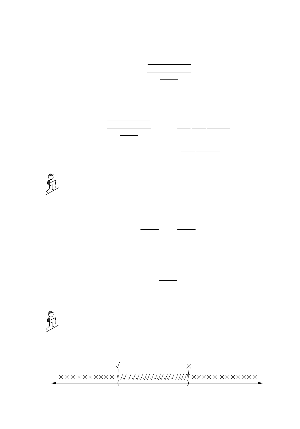
Section 26.1.2: How to find the radius and region of convergence • 555
limits as n → ∞. So we are looking for
lim
n→∞
x
n+1
(n + 1) ln(n + 1)
x
n
n ln(n)
.
This can be dealt with in the same way as ratio test problems for plain vanilla
series: just group together like terms. You get
lim
n→∞
x
n+1
(n + 1) ln(n + 1)
x
n
n ln(n)
= lim
n→∞
x
n+1
x
n
n
n + 1
ln(n)
ln(n + 1)
= lim
n→∞
|x|
n
n + 1
ln(n)
ln(n + 1)
= |x|.
Again, the limit is as n → ∞, which is why we replaced n/(n + 1) and
ln(n)/ ln(n + 1) by 1. (Use l’Hˆopital’s Rule to deal with the logarithms; I’ll
leave the details to you.) Anyway, the limiting ratio is |x|, so by the ratio
PSfrag replacements
(
a, b)
[
a, b]
(
a, b]
[
a, b)
(
a, ∞)
[
a, ∞)
(
−∞, b)
(
−∞, b]
(
−∞, ∞)
{
x : a < x < b}
{
x : a ≤ x ≤ b}
{
x : a < x ≤ b}
{
x : a ≤ x < b}
{
x : x ≥ a}
{
x : x > a}
{
x : x ≤ b}
{
x : x < b}
R
a
b
shadow
0
1
4
−
2
3
−
3
g(
x) = x
2
f(
x) = x
3
g(
x) = x
2
f(
x) = x
3
mirror (
y = x)
f
−
1
(x) =
3
√
x
y = h
(x)
y = h
−
1
(x)
y = (
x − 1)
2
−
1
x
Same height
−
x
Same length,
opposite signs
y = −
2x
−
2
1
y =
1
2
x − 1
2
−
1
y = 2
x
y = 10
x
y = 2
−
x
y = log
2
(
x)
4
3 units
mirror (
x-axis)
y = |
x|
y = |
log
2
(x)|
θ radians
θ units
30
◦
=
π
6
45
◦
=
π
4
60
◦
=
π
3
120
◦
=
2
π
3
135
◦
=
3
π
4
150
◦
=
5
π
6
90
◦
=
π
2
180
◦
= π
210
◦
=
7
π
6
225
◦
=
5
π
4
240
◦
=
4
π
3
270
◦
=
3
π
2
300
◦
=
5
π
3
315
◦
=
7
π
4
330
◦
=
11
π
6
0
◦
= 0 radians
θ
hypotenuse
opposite
adjacent
0 (
≡ 2π)
π
2
π
3
π
2
I
II
III
IV
θ
(
x, y)
x
y
r
7
π
6
reference angle
reference angle =
π
6
sin +
sin −
cos +
cos −
tan +
tan −
A
S
T
C
7
π
4
9
π
13
5
π
6
(this angle is
5
π
6
clockwise)
1
2
1
2
3
4
5
6
0
−
1
−
2
−
3
−
4
−
5
−
6
−
3π
−
5
π
2
−
2π
−
3
π
2
−
π
−
π
2
3
π
3
π
5
π
2
2
π
3
π
2
π
π
2
y = sin(
x)
1
0
−
1
−
3π
−
5
π
2
−
2π
−
3
π
2
−
π
−
π
2
3
π
5
π
2
2
π
2
π
3
π
2
π
π
2
y = sin(
x)
y = cos(
x)
−
π
2
π
2
y = tan(
x), −
π
2
< x <
π
2
0
−
π
2
π
2
y = tan(
x)
−
2π
−
3π
−
5
π
2
−
3
π
2
−
π
−
π
2
π
2
3
π
3
π
5
π
2
2
π
3
π
2
π
y = sec(
x)
y = csc(
x)
y = cot(
x)
y = f(
x)
−
1
1
2
y = g(
x)
3
y = h
(x)
4
5
−
2
f(
x) =
1
x
g(
x) =
1
x
2
etc.
0
1
π
1
2
π
1
3
π
1
4
π
1
5
π
1
6
π
1
7
π
g(
x) = sin
1
x
1
0
−
1
L
10
100
200
y =
π
2
y = −
π
2
y = tan
−
1
(x)
π
2
π
y =
sin(
x)
x
, x > 3
0
1
−
1
a
L
f(
x) = x sin (1/x)
(0 < x < 0
.3)
h
(x) = x
g(
x) = −x
a
L
lim
x
→a
+
f(x) = L
lim
x
→a
+
f(x) = ∞
lim
x
→a
+
f(x) = −∞
lim
x
→a
+
f(x) DNE
lim
x
→a
−
f(x) = L
lim
x
→a
−
f(x) = ∞
lim
x
→a
−
f(x) = −∞
lim
x
→a
−
f(x) DNE
M
}
lim
x
→a
−
f(x) = M
lim
x
→a
f(x) = L
lim
x
→a
f(x) DNE
lim
x
→∞
f(x) = L
lim
x
→∞
f(x) = ∞
lim
x
→∞
f(x) = −∞
lim
x
→∞
f(x) DNE
lim
x
→−∞
f(x) = L
lim
x
→−∞
f(x) = ∞
lim
x
→−∞
f(x) = −∞
lim
x
→−∞
f(x) DNE
lim
x →a
+
f(
x) = ∞
lim
x →a
+
f(
x) = −∞
lim
x →a
−
f(
x) = ∞
lim
x →a
−
f(
x) = −∞
lim
x →a
f(
x) = ∞
lim
x →a
f(
x) = −∞
lim
x →a
f(
x) DNE
y = f (
x)
a
y =
|
x|
x
1
−
1
y =
|
x + 2|
x + 2
1
−
1
−
2
1
2
3
4
a
a
b
y = x sin
1
x
y = x
y = −
x
a
b
c
d
C
a
b
c
d
−
1
0
1
2
3
time
y
t
u
(
t, f(t))
(
u, f(u))
time
y
t
u
y
x
(
x, f(x))
y = |
x|
(
z, f(z))
z
y = f(
x)
a
tangent at x = a
b
tangent at x = b
c
tangent at x = c
y = x
2
tangent
at x = −
1
u
v
uv
u + ∆
u
v + ∆
v
(
u + ∆u)(v + ∆v)
∆
u
∆
v
u
∆v
v∆
u
∆
u∆v
y = f(
x)
1
2
−
2
y = |
x
2
− 4|
y = x
2
− 4
y = −
2x + 5
y = g(
x)
1
2
3
4
5
6
7
8
9
0
−
1
−
2
−
3
−
4
−
5
−
6
y = f (
x)
3
−
3
3
−
3
0
−
1
2
easy
hard
flat
y = f
0
(
x)
3
−
3
0
−
1
2
1
−
1
y = sin(
x)
y = x
x
A
B
O
1
C
D
sin(
x)
tan(
x)
y =
sin(
x)
x
π
2
π
1
−
1
x = 0
a = 0
x > 0
a > 0
x < 0
a < 0
rest position
+
−
y = x
2
sin
1
x
N
A
B
H
a
b
c
O
H
A
B
C
D
h
r
R
θ
1000
2000
α
β
p
h
y = g(
x) = log
b
(x)
y = f(
x) = b
x
y = e
x
5
10
1
2
3
4
0
−
1
−
2
−
3
−
4
y = ln(
x)
y = cosh(
x)
y = sinh(
x)
y = tanh(
x)
y = sech(
x)
y = csch(
x)
y = coth(
x)
1
−
1
y = f(
x)
original function
inverse function
slope = 0 at (
x, y)
slope is infinite at (
y, x)
−
108
2
5
1
2
1
2
3
4
5
6
0
−
1
−
2
−
3
−
4
−
5
−
6
−
3π
−
5
π
2
−
2π
−
3
π
2
−
π
−
π
2
3
π
3
π
5
π
2
2
π
3
π
2
π
π
2
y = sin(
x)
1
0
−
1
−
3π
−
5
π
2
−
2π
−
3
π
2
−
π
−
π
2
3
π
5
π
2
2
π
2
π
3
π
2
π
π
2
y = sin(
x)
y = sin(
x), −
π
2
≤ x ≤
π
2
−
2
−
1
0
2
π
2
−
π
2
y = sin
−
1
(x)
y = cos(
x)
π
π
2
y = cos
−
1
(x)
−
π
2
1
x
α
β
y = tan(
x)
y = tan(
x)
1
y = tan
−
1
(x)
y = sec(
x)
y = sec
−
1
(x)
y = csc
−
1
(x)
y = cot
−
1
(x)
1
y = cosh
−
1
(x)
y = sinh
−
1
(x)
y = tanh
−
1
(x)
y = sech
−
1
(x)
y = csch
−
1
(x)
y = coth
−
1
(x)
(0
, 3)
(2
, −1)
(5
, 2)
(7
, 0)
(
−1, 44)
(0
, 1)
(1
, −12)
(2
, 305)
y = 1
2
(2
, 3)
y = f(
x)
y = g(
x)
a
b
c
a
b
c
s
c
0
c
1
(
a, f(a))
(
b, f(b))
1
2
1
2
3
4
5
6
0
−
1
−
2
−
3
−
4
−
5
−
6
−
3π
−
5
π
2
−
2π
−
3
π
2
−
π
−
π
2
3
π
3
π
5
π
2
2
π
3
π
2
π
π
2
y = sin(
x)
1
0
−
1
−
3π
−
5
π
2
−
2π
−
3
π
2
−
π
−
π
2
3
π
5
π
2
2
π
2
π
3
π
2
π
π
2
c
OR
Local maximum
Local minimum
Horizontal point of inflection
1
e
y = f
0
(
x)
y = f (
x) = x ln(x)
−
1
e
?
y = f(
x) = x
3
y = g(
x) = x
4
x
f(
x)
−
3
−
2
−
1
0
1
2
1
2
3
4
+
−
?
1
5
6
3
f
0
(
x)
2 −
1
2
√
6
2 +
1
2
√
6
f
00
(
x)
7
8
g
00
(
x)
f
00
(
x)
0
y =
(
x − 3)(x − 1)
2
x
3
(
x + 2)
y = x ln(
x)
1
e
−
1
e
5
−
108
2
α
β
2 −
1
2
√
6
2 +
1
2
√
6
y = x
2
(
x − 5)
3
−
e
−
1/2
√
3
e
−
1/2
√
3
−
e
−3/2
e
−
3/2
−
1
√
3
1
√
3
−
1
1
y = xe
−
3x
2
/2
y =
x
3
− 6
x
2
+ 13x − 8
x
28
2
600
500
400
300
200
100
0
−
100
−
200
−
300
−
400
−
500
−
600
0
10
−
10
5
−
5
20
−
20
15
−
15
0
4
5
6
x
P
0
(
x)
+
−
−
existing fence
new fence
enclosure
A
h
b
H
99
100
101
h
dA/dh
r
h
1
2
7
shallow
deep
LAND
SEA
N
y
z
s
t
3
11
9
L
(11)
√
11
y = L
(x)
y = f (
x)
11
y = L
(x)
y = f(
x)
F
P
a
a + ∆
x
f(
a + ∆x)
L
(a + ∆x)
f(
a)
error
df
∆
x
a
b
y = f(
x)
true zero
starting approximation
better approximation
v
t
3
5
50
40
60
4
20
30
25
t
1
t
2
t
3
t
4
t
n
−2
t
n
−1
t
0
= a
t
n
= b
v
1
v
2
v
3
v
4
v
n
−1
v
n
−
30
6
30
|
v|
a
b
p
q
c
v(
c)
v(
c
1
)
v(
c
2
)
v(
c
3
)
v(
c
4
)
v(
c
5
)
v(
c
6
)
t
1
t
2
t
3
t
4
t
5
c
1
c
2
c
3
c
4
c
5
c
6
t
0
=
a
t
6
=
b
t
16
=
b
t
10
=
b
a
b
x
y
y = f(
x)
1
2
y = x
5
0
−
2
y = 1
a
b
y = sin(
x)
π
−
π
0
−
1
−
2
0
2
4
y = x
2
0
1
2
3
4
2
n
4
n
6
n
2(
n−2)
n
2(
n−1)
n
2
n
n
= 2
width of each interval =
2
n
−
2
1
3
0
I
II
III
IV
4
y
dx
y = −
x
2
− 2x + 3
3
−
5
y = |−
x
2
− 2x + 3|
I
II
IIa
5
3
0
1
2
a
b
y = f (
x)
y = g(
x)
y = x
2
a
b
5
3
0
1
2
y =
√
x
2
√
2
2
2
dy
x
2
a
b
y = f(
x)
y = g(
x)
M
m
1
2
−
1
−
2
0
y = e
−
x
2
1
2
e
−
1/4
f
av
y = f
av
c
A
M
0
1
2
a
b
x
t
y = f (
t)
F (
x )
y = f (
t)
F (
x + h)
x + h
F (
x + h) − F (x)
f(
x)
1
2
y = sin(
x)
π
−
π
−
1
−
2
y =
1
x
y = x
2
1
2
1
−
1
y = ln
|x|
θ
a
x
a
x
p
a
2
− x
2
3
x
p
9 − x
2
p
x
2
+ a
2
x
a
p
x
2
+ 15
x
√
15
x
p
x
2
− a
2
a
x
p
x
2
− 4
2
x
−
p
x
2
− a
2
a
x
−
p
x
2
− 4
2
y = f(x)
a
b
a + ε
ε
Z
b
a+ε
f(x) dx
small
even smaller
y = g(x)
infinite area
finite area
1
y =
1
x
y =
1
x
p
, p < 1 (typical)
y =
1
x
p
, p > 1 (typical)
a
1
a
2
a
3
a
4
a
5
a
6
a
7
a
8
1
2
3
4
5
6
7
8
n
a
n
x
y
y = f(x)
(a, f(a))
a
−1
0
1
a
test, our power series converges absolutely when |x| < 1 and diverges when
|x| > 1. That is, the radius of convergence is 1. We still have to check what
happens when x = 1 and x = −1. Let’s do x = 1 first. Substituting x = 1,
the original power series becomes
∞
X
n=2
1
n
n ln(n)
=
∞
X
n=2
1
n ln(n)
.
Does this converge? I leave it to you to use the integral test to see that it
diverges (or see Section 23.5 in Chapter 23). Now let’s put x = −1 in the
original power series above to get
∞
X
n=2
(−1)
n
n ln(n)
.
This doesn’t converge absolutely—in fact, the series obtained by replacing
the terms by their absolute values is exactly the series when x = 1, which we
just saw diverges. On the other hand, the above series for x = −1 converges
by the alternating series test (you supply the details—use the methods of
PSfrag replacements
(
a, b)
[
a, b]
(
a, b]
[
a, b)
(
a, ∞)
[
a, ∞)
(
−∞, b)
(
−∞, b]
(
−∞, ∞)
{
x : a < x < b}
{
x : a ≤ x ≤ b}
{
x : a < x ≤ b}
{
x : a ≤ x < b}
{
x : x ≥ a}
{
x : x > a}
{
x : x ≤ b}
{
x : x < b}
R
a
b
shadow
0
1
4
−
2
3
−
3
g(
x) = x
2
f(
x) = x
3
g(
x) = x
2
f(
x) = x
3
mirror (
y = x)
f
−
1
(x) =
3
√
x
y = h
(x)
y = h
−
1
(x)
y = (
x − 1)
2
−
1
x
Same height
−
x
Same length,
opposite signs
y = −
2x
−
2
1
y =
1
2
x − 1
2
−
1
y = 2
x
y = 10
x
y = 2
−
x
y = log
2
(
x)
4
3 units
mirror (
x-axis)
y = |
x|
y = |
log
2
(x)|
θ radians
θ units
30
◦
=
π
6
45
◦
=
π
4
60
◦
=
π
3
120
◦
=
2
π
3
135
◦
=
3
π
4
150
◦
=
5
π
6
90
◦
=
π
2
180
◦
= π
210
◦
=
7
π
6
225
◦
=
5
π
4
240
◦
=
4
π
3
270
◦
=
3
π
2
300
◦
=
5
π
3
315
◦
=
7
π
4
330
◦
=
11
π
6
0
◦
= 0 radians
θ
hypotenuse
opposite
adjacent
0 (
≡ 2π)
π
2
π
3
π
2
I
II
III
IV
θ
(
x, y)
x
y
r
7
π
6
reference angle
reference angle =
π
6
sin +
sin −
cos +
cos −
tan +
tan −
A
S
T
C
7
π
4
9
π
13
5
π
6
(this angle is
5
π
6
clockwise)
1
2
1
2
3
4
5
6
0
−
1
−
2
−
3
−
4
−
5
−
6
−
3π
−
5
π
2
−
2π
−
3
π
2
−
π
−
π
2
3
π
3
π
5
π
2
2
π
3
π
2
π
π
2
y = sin(
x)
1
0
−
1
−
3π
−
5
π
2
−
2π
−
3
π
2
−
π
−
π
2
3
π
5
π
2
2
π
2
π
3
π
2
π
π
2
y = sin(
x)
y = cos(
x)
−
π
2
π
2
y = tan(
x), −
π
2
< x <
π
2
0
−
π
2
π
2
y = tan(
x)
−
2π
−
3π
−
5
π
2
−
3
π
2
−
π
−
π
2
π
2
3
π
3
π
5
π
2
2
π
3
π
2
π
y = sec(
x)
y = csc(
x)
y = cot(
x)
y = f(
x)
−
1
1
2
y = g(
x)
3
y = h
(x)
4
5
−
2
f(
x) =
1
x
g(
x) =
1
x
2
etc.
0
1
π
1
2
π
1
3
π
1
4
π
1
5
π
1
6
π
1
7
π
g(
x) = sin
1
x
1
0
−
1
L
10
100
200
y =
π
2
y = −
π
2
y = tan
−
1
(x)
π
2
π
y =
sin(
x)
x
, x > 3
0
1
−
1
a
L
f(
x) = x sin (1/x)
(0 < x < 0
.3)
h
(x) = x
g(
x) = −x
a
L
lim
x
→a
+
f(x) = L
lim
x
→a
+
f(x) = ∞
lim
x
→a
+
f(x) = −∞
lim
x
→a
+
f(x) DNE
lim
x
→a
−
f(x) = L
lim
x
→a
−
f(x) = ∞
lim
x
→a
−
f(x) = −∞
lim
x
→a
−
f(x) DNE
M
}
lim
x
→a
−
f(x) = M
lim
x
→a
f(x) = L
lim
x
→a
f(x) DNE
lim
x
→∞
f(x) = L
lim
x
→∞
f(x) = ∞
lim
x
→∞
f(x) = −∞
lim
x
→∞
f(x) DNE
lim
x
→−∞
f(x) = L
lim
x
→−∞
f(x) = ∞
lim
x
→−∞
f(x) = −∞
lim
x
→−∞
f(x) DNE
lim
x →a
+
f(
x) = ∞
lim
x →a
+
f(
x) = −∞
lim
x →a
−
f(
x) = ∞
lim
x →a
−
f(
x) = −∞
lim
x →a
f(
x) = ∞
lim
x →a
f(
x) = −∞
lim
x →a
f(
x) DNE
y = f (
x)
a
y =
|
x|
x
1
−
1
y =
|
x + 2|
x + 2
1
−
1
−
2
1
2
3
4
a
a
b
y = x sin
1
x
y = x
y = −
x
a
b
c
d
C
a
b
c
d
−
1
0
1
2
3
time
y
t
u
(
t, f(t))
(
u, f(u))
time
y
t
u
y
x
(
x, f(x))
y = |
x|
(
z, f(z))
z
y = f(
x)
a
tangent at x = a
b
tangent at x = b
c
tangent at x = c
y = x
2
tangent
at x = −
1
u
v
uv
u + ∆
u
v + ∆
v
(
u + ∆u)(v + ∆v)
∆
u
∆
v
u
∆v
v∆
u
∆
u∆v
y = f(
x)
1
2
−
2
y = |
x
2
− 4|
y = x
2
− 4
y = −
2x + 5
y = g(
x)
1
2
3
4
5
6
7
8
9
0
−
1
−
2
−
3
−
4
−
5
−
6
y = f (
x)
3
−
3
3
−
3
0
−
1
2
easy
hard
flat
y = f
0
(
x)
3
−
3
0
−
1
2
1
−
1
y = sin(
x)
y = x
x
A
B
O
1
C
D
sin(
x)
tan(
x)
y =
sin(
x)
x
π
2
π
1
−
1
x = 0
a = 0
x > 0
a > 0
x < 0
a < 0
rest position
+
−
y = x
2
sin
1
x
N
A
B
H
a
b
c
O
H
A
B
C
D
h
r
R
θ
1000
2000
α
β
p
h
y = g(
x) = log
b
(x)
y = f(
x) = b
x
y = e
x
5
10
1
2
3
4
0
−
1
−
2
−
3
−
4
y = ln(
x)
y = cosh(
x)
y = sinh(
x)
y = tanh(
x)
y = sech(
x)
y = csch(
x)
y = coth(
x)
1
−
1
y = f(
x)
original function
inverse function
slope = 0 at (
x, y)
slope is infinite at (
y, x)
−
108
2
5
1
2
1
2
3
4
5
6
0
−
1
−
2
−
3
−
4
−
5
−
6
−
3π
−
5
π
2
−
2π
−
3
π
2
−
π
−
π
2
3
π
3
π
5
π
2
2
π
3
π
2
π
π
2
y = sin(
x)
1
0
−
1
−
3π
−
5
π
2
−
2π
−
3
π
2
−
π
−
π
2
3
π
5
π
2
2
π
2
π
3
π
2
π
π
2
y = sin(
x)
y = sin(
x), −
π
2
≤ x ≤
π
2
−
2
−
1
0
2
π
2
−
π
2
y = sin
−
1
(x)
y = cos(
x)
π
π
2
y = cos
−
1
(x)
−
π
2
1
x
α
β
y = tan(
x)
y = tan(
x)
1
y = tan
−
1
(x)
y = sec(
x)
y = sec
−
1
(x)
y = csc
−
1
(x)
y = cot
−
1
(x)
1
y = cosh
−
1
(x)
y = sinh
−
1
(x)
y = tanh
−
1
(x)
y = sech
−
1
(x)
y = csch
−
1
(x)
y = coth
−
1
(x)
(0
, 3)
(2
, −1)
(5
, 2)
(7
, 0)
(
−1, 44)
(0
, 1)
(1
, −12)
(2
, 305)
y = 1
2
(2
, 3)
y = f(
x)
y = g(
x)
a
b
c
a
b
c
s
c
0
c
1
(
a, f(a))
(
b, f(b))
1
2
1
2
3
4
5
6
0
−
1
−
2
−
3
−
4
−
5
−
6
−
3π
−
5
π
2
−
2π
−
3
π
2
−
π
−
π
2
3
π
3
π
5
π
2
2
π
3
π
2
π
π
2
y = sin(
x)
1
0
−
1
−
3π
−
5
π
2
−
2π
−
3
π
2
−
π
−
π
2
3
π
5
π
2
2
π
2
π
3
π
2
π
π
2
c
OR
Local maximum
Local minimum
Horizontal point of inflection
1
e
y = f
0
(
x)
y = f (
x) = x ln(x)
−
1
e
?
y = f(
x) = x
3
y = g(
x) = x
4
x
f(
x)
−
3
−
2
−
1
0
1
2
1
2
3
4
+
−
?
1
5
6
3
f
0
(
x)
2 −
1
2
√
6
2 +
1
2
√
6
f
00
(
x)
7
8
g
00
(
x)
f
00
(
x)
0
y =
(
x − 3)(x − 1)
2
x
3
(
x + 2)
y = x ln(
x)
1
e
−
1
e
5
−
108
2
α
β
2 −
1
2
√
6
2 +
1
2
√
6
y = x
2
(
x − 5)
3
−
e
−
1/2
√
3
e
−
1/2
√
3
−
e
−3/2
e
−
3/2
−
1
√
3
1
√
3
−
1
1
y = xe
−
3x
2
/2
y =
x
3
− 6
x
2
+ 13x − 8
x
28
2
600
500
400
300
200
100
0
−
100
−
200
−
300
−
400
−
500
−
600
0
10
−
10
5
−
5
20
−
20
15
−
15
0
4
5
6
x
P
0
(
x)
+
−
−
existing fence
new fence
enclosure
A
h
b
H
99
100
101
h
dA/dh
r
h
1
2
7
shallow
deep
LAND
SEA
N
y
z
s
t
3
11
9
L
(11)
√
11
y = L
(x)
y = f (
x)
11
y = L
(x)
y = f(
x)
F
P
a
a + ∆
x
f(
a + ∆x)
L
(a + ∆x)
f(
a)
error
df
∆
x
a
b
y = f(
x)
true zero
starting approximation
better approximation
v
t
3
5
50
40
60
4
20
30
25
t
1
t
2
t
3
t
4
t
n
−2
t
n
−1
t
0
= a
t
n
= b
v
1
v
2
v
3
v
4
v
n
−1
v
n
−
30
6
30
|
v|
a
b
p
q
c
v(
c)
v(
c
1
)
v(
c
2
)
v(
c
3
)
v(
c
4
)
v(
c
5
)
v(
c
6
)
t
1
t
2
t
3
t
4
t
5
c
1
c
2
c
3
c
4
c
5
c
6
t
0
=
a
t
6
=
b
t
16
=
b
t
10
=
b
a
b
x
y
y = f(
x)
1
2
y = x
5
0
−
2
y = 1
a
b
y = sin(
x)
π
−
π
0
−
1
−
2
0
2
4
y = x
2
0
1
2
3
4
2
n
4
n
6
n
2(
n−2)
n
2(
n−1)
n
2
n
n
= 2
width of each interval =
2
n
−
2
1
3
0
I
II
III
IV
4
y
dx
y = −
x
2
− 2x + 3
3
−
5
y = |−
x
2
− 2x + 3|
I
II
IIa
5
3
0
1
2
a
b
y = f (
x)
y = g(
x)
y = x
2
a
b
5
3
0
1
2
y =
√
x
2
√
2
2
2
dy
x
2
a
b
y = f(
x)
y = g(
x)
M
m
1
2
−
1
−
2
0
y = e
−
x
2
1
2
e
−
1/4
f
av
y = f
av
c
A
M
0
1
2
a
b
x
t
y = f (
t)
F (
x )
y = f (
t)
F (
x + h)
x + h
F (
x + h) − F (x)
f(
x)
1
2
y = sin(
x)
π
−
π
−
1
−
2
y =
1
x
y = x
2
1
2
1
−1
y = ln|x|
θ
a
x
a
x
p
a
2
− x
2
3
x
p
9 − x
2
p
x
2
+ a
2
x
a
p
x
2
+ 15
x
√
15
x
p
x
2
− a
2
a
x
p
x
2
− 4
2
x
−
p
x
2
− a
2
a
x
−
p
x
2
− 4
2
y = f(x)
a
b
a + ε
ε
Z
b
a+ε
f(x) dx
small
even smaller
y = g(x)
infinite area
finite area
1
y =
1
x
y =
1
x
p
, p < 1 (typical)
y =
1
x
p
, p > 1 (typical)
a
1
a
2
a
3
a
4
a
5
a
6
a
7
a
8
1
2
3
4
5
6
7
8
n
a
n
x
y
y = f(x)
(a, f(a))
a
−1
0
1
a
Section 23.7 of Chapter 23). So, we have conditional convergence at the
point x = −1. Summarizing, the power series converges absolutely when
−1 < x < 1, converges conditionally when x = −1, and diverges for all other
x. The picture looks like this:
PSfrag replacements
(
a, b)
[
a, b]
(
a, b]
[
a, b)
(
a, ∞)
[
a, ∞)
(
−∞, b)
(
−∞, b]
(
−∞, ∞)
{
x : a < x < b}
{
x : a ≤ x ≤ b}
{
x : a < x ≤ b}
{
x : a ≤ x < b}
{
x : x ≥ a}
{
x : x > a}
{
x : x ≤ b}
{
x : x < b}
R
a
b
shadow
0
1
4
−
2
3
−
3
g(
x) = x
2
f(
x) = x
3
g(
x) = x
2
f(
x) = x
3
mirror (
y = x)
f
−
1
(x) =
3
√
x
y = h
(x)
y = h
−
1
(x)
y = (
x − 1)
2
−
1
x
Same height
−
x
Same length,
opposite signs
y = −
2x
−
2
1
y =
1
2
x − 1
2
−
1
y = 2
x
y = 10
x
y = 2
−
x
y = log
2
(
x)
4
3 units
mirror (
x-axis)
y = |
x|
y = |
log
2
(x)|
θ radians
θ units
30
◦
=
π
6
45
◦
=
π
4
60
◦
=
π
3
120
◦
=
2
π
3
135
◦
=
3
π
4
150
◦
=
5
π
6
90
◦
=
π
2
180
◦
= π
210
◦
=
7
π
6
225
◦
=
5
π
4
240
◦
=
4
π
3
270
◦
=
3
π
2
300
◦
=
5
π
3
315
◦
=
7
π
4
330
◦
=
11
π
6
0
◦
= 0 radians
θ
hypotenuse
opposite
adjacent
0 (
≡ 2π)
π
2
π
3
π
2
I
II
III
IV
θ
(
x, y)
x
y
r
7
π
6
reference angle
reference angle =
π
6
sin +
sin −
cos +
cos −
tan +
tan −
A
S
T
C
7
π
4
9
π
13
5
π
6
(this angle is
5
π
6
clockwise)
1
2
1
2
3
4
5
6
0
−
1
−
2
−
3
−
4
−
5
−
6
−
3π
−
5
π
2
−
2π
−
3
π
2
−
π
−
π
2
3
π
3
π
5
π
2
2
π
3
π
2
π
π
2
y = sin(
x)
1
0
−
1
−
3π
−
5
π
2
−
2π
−
3
π
2
−
π
−
π
2
3
π
5
π
2
2
π
2
π
3
π
2
π
π
2
y = sin(
x)
y = cos(
x)
−
π
2
π
2
y = tan(
x), −
π
2
< x <
π
2
0
−
π
2
π
2
y = tan(
x)
−
2π
−
3π
−
5
π
2
−
3
π
2
−
π
−
π
2
π
2
3
π
3
π
5
π
2
2
π
3
π
2
π
y = sec(
x)
y = csc(
x)
y = cot(
x)
y = f(
x)
−
1
1
2
y = g(
x)
3
y = h
(x)
4
5
−
2
f(
x) =
1
x
g(
x) =
1
x
2
etc.
0
1
π
1
2
π
1
3
π
1
4
π
1
5
π
1
6
π
1
7
π
g(
x) = sin
1
x
1
0
−
1
L
10
100
200
y =
π
2
y = −
π
2
y = tan
−
1
(x)
π
2
π
y =
sin(
x)
x
, x > 3
0
1
−
1
a
L
f(
x) = x sin (1/x)
(0 < x < 0
.3)
h
(x) = x
g(
x) = −x
a
L
lim
x
→a
+
f(x) = L
lim
x
→a
+
f(x) = ∞
lim
x
→a
+
f(x) = −∞
lim
x
→a
+
f(x) DNE
lim
x
→a
−
f(x) = L
lim
x
→a
−
f(x) = ∞
lim
x
→a
−
f(x) = −∞
lim
x
→a
−
f(x) DNE
M
}
lim
x
→a
−
f(x) = M
lim
x
→a
f(x) = L
lim
x
→a
f(x) DNE
lim
x
→∞
f(x) = L
lim
x
→∞
f(x) = ∞
lim
x
→∞
f(x) = −∞
lim
x
→∞
f(x) DNE
lim
x
→−∞
f(x) = L
lim
x
→−∞
f(x) = ∞
lim
x
→−∞
f(x) = −∞
lim
x
→−∞
f(x) DNE
lim
x →a
+
f(
x) = ∞
lim
x →a
+
f(
x) = −∞
lim
x →a
−
f(
x) = ∞
lim
x →a
−
f(
x) = −∞
lim
x →a
f(
x) = ∞
lim
x →a
f(
x) = −∞
lim
x →a
f(
x) DNE
y = f (
x)
a
y =
|
x|
x
1
−
1
y =
|
x + 2|
x + 2
1
−
1
−
2
1
2
3
4
a
a
b
y = x sin
1
x
y = x
y = −
x
a
b
c
d
C
a
b
c
d
−
1
0
1
2
3
time
y
t
u
(
t, f(t))
(
u, f(u))
time
y
t
u
y
x
(
x, f(x))
y = |
x|
(
z, f(z))
z
y = f(
x)
a
tangent at x = a
b
tangent at x = b
c
tangent at x = c
y = x
2
tangent
at x = −
1
u
v
uv
u + ∆
u
v + ∆
v
(
u + ∆u)(v + ∆v)
∆
u
∆
v
u
∆v
v∆
u
∆
u∆v
y = f(
x)
1
2
−
2
y = |
x
2
− 4|
y = x
2
− 4
y = −
2x + 5
y = g(
x)
1
2
3
4
5
6
7
8
9
0
−
1
−
2
−
3
−
4
−
5
−
6
y = f (
x)
3
−
3
3
−
3
0
−
1
2
easy
hard
flat
y = f
0
(
x)
3
−
3
0
−
1
2
1
−
1
y = sin(
x)
y = x
x
A
B
O
1
C
D
sin(
x)
tan(
x)
y =
sin(
x)
x
π
2
π
1
−
1
x = 0
a = 0
x > 0
a > 0
x < 0
a < 0
rest position
+
−
y = x
2
sin
1
x
N
A
B
H
a
b
c
O
H
A
B
C
D
h
r
R
θ
1000
2000
α
β
p
h
y = g(
x) = log
b
(x)
y = f(
x) = b
x
y = e
x
5
10
1
2
3
4
0
−
1
−
2
−
3
−
4
y = ln(
x)
y = cosh(
x)
y = sinh(
x)
y = tanh(
x)
y = sech(
x)
y = csch(
x)
y = coth(
x)
1
−
1
y = f(
x)
original function
inverse function
slope = 0 at (
x, y)
slope is infinite at (
y, x)
−
108
2
5
1
2
1
2
3
4
5
6
0
−
1
−
2
−
3
−
4
−
5
−
6
−
3π
−
5
π
2
−
2π
−
3
π
2
−
π
−
π
2
3
π
3
π
5
π
2
2
π
3
π
2
π
π
2
y = sin(
x)
1
0
−
1
−
3π
−
5
π
2
−
2π
−
3
π
2
−
π
−
π
2
3
π
5
π
2
2
π
2
π
3
π
2
π
π
2
y = sin(
x)
y = sin(
x), −
π
2
≤ x ≤
π
2
−
2
−
1
0
2
π
2
−
π
2
y = sin
−
1
(x)
y = cos(
x)
π
π
2
y = cos
−
1
(x)
−
π
2
1
x
α
β
y = tan(
x)
y = tan(
x)
1
y = tan
−
1
(x)
y = sec(
x)
y = sec
−
1
(x)
y = csc
−
1
(x)
y = cot
−
1
(x)
1
y = cosh
−
1
(x)
y = sinh
−
1
(x)
y = tanh
−
1
(x)
y = sech
−
1
(x)
y = csch
−
1
(x)
y = coth
−
1
(x)
(0
, 3)
(2
, −1)
(5
, 2)
(7
, 0)
(
−1, 44)
(0
, 1)
(1
, −12)
(2
, 305)
y = 1
2
(2
, 3)
y = f(
x)
y = g(
x)
a
b
c
a
b
c
s
c
0
c
1
(
a, f(a))
(
b, f(b))
1
2
1
2
3
4
5
6
0
−
1
−
2
−
3
−
4
−
5
−
6
−
3π
−
5
π
2
−
2π
−
3
π
2
−
π
−
π
2
3
π
3
π
5
π
2
2
π
3
π
2
π
π
2
y = sin(
x)
1
0
−
1
−
3π
−
5
π
2
−
2π
−
3
π
2
−
π
−
π
2
3
π
5
π
2
2
π
2
π
3
π
2
π
π
2
c
OR
Local maximum
Local minimum
Horizontal point of inflection
1
e
y = f
0
(
x)
y = f (
x) = x ln(x)
−
1
e
?
y = f(
x) = x
3
y = g(
x) = x
4
x
f(
x)
−
3
−
2
−
1
0
1
2
1
2
3
4
+
−
?
1
5
6
3
f
0
(
x)
2 −
1
2
√
6
2 +
1
2
√
6
f
00
(
x)
7
8
g
00
(
x)
f
00
(
x)
0
y =
(
x − 3)(x − 1)
2
x
3
(
x + 2)
y = x ln(
x)
1
e
−
1
e
5
−
108
2
α
β
2 −
1
2
√
6
2 +
1
2
√
6
y = x
2
(
x − 5)
3
−
e
−
1/2
√
3
e
−
1/2
√
3
−
e
−3/2
e
−
3/2
−
1
√
3
1
√
3
−
1
1
y = xe
−
3x
2
/2
y =
x
3
− 6
x
2
+ 13x − 8
x
28
2
600
500
400
300
200
100
0
−
100
−
200
−
300
−
400
−
500
−
600
0
10
−
10
5
−
5
20
−
20
15
−
15
0
4
5
6
x
P
0
(
x)
+
−
−
existing fence
new fence
enclosure
A
h
b
H
99
100
101
h
dA/dh
r
h
1
2
7
shallow
deep
LAND
SEA
N
y
z
s
t
3
11
9
L
(11)
√
11
y = L
(x)
y = f (
x)
11
y = L
(x)
y = f(
x)
F
P
a
a + ∆
x
f(
a + ∆x)
L
(a + ∆x)
f(
a)
error
df
∆
x
a
b
y = f(
x)
true zero
starting approximation
better approximation
v
t
3
5
50
40
60
4
20
30
25
t
1
t
2
t
3
t
4
t
n
−2
t
n
−1
t
0
= a
t
n
= b
v
1
v
2
v
3
v
4
v
n
−1
v
n
−
30
6
30
|
v|
a
b
p
q
c
v(
c)
v(
c
1
)
v(
c
2
)
v(
c
3
)
v(
c
4
)
v(
c
5
)
v(
c
6
)
t
1
t
2
t
3
t
4
t
5
c
1
c
2
c
3
c
4
c
5
c
6
t
0
=
a
t
6
=
b
t
16
=
b
t
10
=
b
a
b
x
y
y = f(
x)
1
2
y = x
5
0
−
2
y = 1
a
b
y = sin(
x)
π
−
π
0
−
1
−
2
0
2
4
y = x
2
0
1
2
3
4
2
n
4
n
6
n
2(
n−2)
n
2(
n−1)
n
2
n
n
= 2
width of each interval =
2
n
−
2
1
3
0
I
II
III
IV
4
y
dx
y = −
x
2
− 2x + 3
3
−
5
y = |−
x
2
− 2x + 3|
I
II
IIa
5
3
0
1
2
a
b
y = f (
x)
y = g(
x)
y = x
2
a
b
5
3
0
1
2
y =
√
x
2
√
2
2
2
dy
x
2
a
b
y = f(
x)
y = g(
x)
M
m
1
2
−
1
−
2
0
y = e
−
x
2
1
2
e
−
1/4
f
av
y = f
av
c
A
M
0
1
2
a
b
x
t
y = f(
t)
F (
x )
y = f(
t)
F (
x + h)
x + h
F (
x + h) − F (x)
f(x)
1
2
y = sin(x)
π
−π
−1
−2
y =
1
x
y = x
2
1
2
1
−1
y = ln|x|
θ
a
x
a
x
p
a
2
− x
2
3
x
p
9 − x
2
p
x
2
+ a
2
x
a
p
x
2
+ 15
x
√
15
x
p
x
2
− a
2
a
x
p
x
2
− 4
2
x
−
p
x
2
− a
2
a
x
−
p
x
2
− 4
2
y = f(x)
a
b
a + ε
ε
Z
b
a+ε
f(x) dx
small
even smaller
y = g(x)
infinite area
finite area
1
y =
1
x
y =
1
x
p
, p < 1 (typical)
y =
1
x
p
, p > 1 (typical)
a
1
a
2
a
3
a
4
a
5
a
6
a
7
a
8
1
2
3
4
5
6
7
8
n
a
n
x
y
y = f(x)
(a, f(a))
a
−1
0
1
a