Asai K. (ed.) Human-Computer Interaction. New Developments
Подождите немного. Документ загружается.


Miniaturized 3D Human Motion Input
241
4. Outlook
This chapter has outlined the requirements for creating a miniature 3D controller that is
suitable for mobile computing applications, and presented the key elements of the design of
a device fulfilling these requirements. Its key feature is a novel mechanism that provides for
full 6 DOF motion using only one moving part, combined with standard image processing.
While its feasibility has been demonstrated, several improvements are required to achieve a
truly usable mobile controller. The two key necessary improvements include:
• Redesign the imaging device packaging and optics to reduce the depth of the
controller within the case from >40 mm to <15 mm, so that it can fit inside a typical
mobile computing device.
• Find methods for producing the out-of-plane calibration point, probably using
machining or plastic molding, so that full 6 DOF output can be supported instead
of the current 4 DOF.
More straightforward improvements include further optimization of the spring design,
increasing the stiffness of the casing to reduce zero-position hysteresis, and a switch to
higher resolution imagers. Using a 1.3 megapixel imager would improve sensitivity by
approximately 2 bits, at the cost of increasing image processing requirements. It would thus
be desirable to create an embedded version of the vision processing algorithm to create a
stand-alone, platform-independent device with minimal power consumption. Direct
usability comparisons comparing the presented device with existing devices are also
needed.
5. Acknowledgments
Thanks to Rodney Douglas and Wolfgang Henggeler for their advice and encouragement
during the development of the device, and to Adrian Whatley for his corrections to the
manuscript.
6. References
ARToolworks. (2007). ARTookit, from http://www.hitl.washington.edu/artoolkit/.
Bidiville, M., Arreguit, J., van Schaik, F. A., Steenis, B., Droz-Dit-Busset, F., Buczek, H. and
Bussien, A. (1994). Cursor pointing device utilizing a photodetector array with target ball
having randomly distributed speckles. United States Patent and Trademarks Office.
United States of America.
Bisset, S. J. and Kasser, B. (1998). Touch Pad with Scroll Bar, Command Bar. WO 98/37506.
WIPO, Logitech, Inc.
Eng, K. (2007). A Miniature, One-Handed 3D Motion Controller. LNCS4662 Part 1: Interact
2007, Rio de Janeiro, Brasil.
Gombert, B. (2004). Arrangement for the detection for relative movements or relative position of two
objects. US6804012. USA, 3DConnexion GmbH, Seefeld (DE).
Woods, E., Mason, P. and Billinghurst, M. (2003). MagicMouse: an Inexpensive 6-Degree-of-
Freedom Mouse. Proceedings of the 1st international conference on Computer

Human-Computer Interaction, New Developments
242
graphics and interactive techniques in Australasia and South East Asia, Melbourne,
AU, ACM Press.
13
Modeling Query Events in Spoken Natural
Language for Human-Database Interaction
Omar U. Florez and SeungJin Lim
Computer Science Department
Utah Sate University
Logan, UT 84322-4205, USA
1. Introduction
The database-related technologies have been extensively developed over the past decades
and are used widely in modern society. In response to the increasing demands upon high
performing database interaction, many efforts have been made to improve database system
performance. For example, indexing technologies enable us to efficiently retrieve
information from very large databases [1]. However, the user interfaces to database systems
essentially remain unchanged: SQL is the de facto standard language used either directly or
indirectly through an API layer. It is, however, interesting to note that the most common
mode of human interface is the communication through a natural language, which
motivates us to use a natural language as a human-database interface [2]. Let us compare
SQL and natural language in a database query.
– While a query in natural language expresses the mental representation of the goal by the
user, an SQL expression describes the structure of the data stored in the database [3].
– While SQL is a declarative language to describe a fixed set of actions to manipulate data in
a relational database, the set of actions supported by the verbs in a natural language [4] is
large and can be extended.
– Nevertheless, the primary user intention of data manipulation is the same both in SQL and
natural language.
Clearly, there is an important gap to be filled between the cognitive model of the user
interaction with databases by humans in natural language and the structured model in SQL.
This gap represents the different layers of the abstraction of the user interaction carried out
by the user and by the database system over the data. In this work, we attempt to bridge the
gap between spoken natural language and SQL to enable the user to interact with the
database through a voice interface. This goal is achieved by recognizing a query event, whose
structural complexity is moderate, presented in a spoken natural language phrase, and then
translating it to an SQL query. The presence of a query event in a spoken language
expression is detected in our approach by recognizing linguistic patterns in which a verb
triggers a query action followed by a set of words which specify the action. In other words,
our approach works as a linguistic adapter which converts the structure of the spoken
language expression to that of SQL at three different abstraction layers: lexical, syntactic,

244 Human-Computer Interaction, New Developments
and semantic. The structure to be identified and the corresponding actions involved in these
three layers are summarized in Table 1. They will be discussed in depth in later sections.
Abstraction
layer
Spoken natural
language
Actions to bridge
natural
language and SQL
SQL
Lexical Voice signal from
the
user
Detection of
phonemes
from the voice signal
and
word formation
from the
phonemes
Words
Syntactic Parts of speech of
words
by the proposed
grammar
Syntactic analysis of
parts of speech
Keywords and
literals by
the SQL
grammar
Semantic Queries in natural
language
Representation of
queries
as events in a word
stream
No meta data or
events
are considered.
Syntactically
valid actions are
to
be executed.
Table 1: The characteristics of the three linguistic abstraction layers in spoken natural
language and SQL.
There are a wide range of interesting applications that can benefit from the proposed spoken
language-based database interaction, ranging from an alternative user interface to perform
database queries to voice-enabled retrieval of medical images in surgery. To this end, our
contribution to the study of human-computer interaction is threefold. First, we formalize the
detection of the presence of database queries in the user speech by modeling them as special
events over time, called query events. Second, we provide a mechanism to translate a query
event in a spoken natural language to an SQL query. Finally, we developed an application
prototype, called Voice2SQL, to demonstrate the proposed user-database interaction
approach in an application.
2. Previous Work
The work to enhance the interaction between humans and database systems has evolved
over time. The approaches that are found in the literature can be classified into two by the
way in which the interaction is carried on: textual and visual. While the use interaction in
textual query systems (TQS) consists of typing SQL sentences using a keyboard, in visual

Modeling Query Events in Spoken Natural Language for Human-Database Interaction 245
query systems (VQS) the human interaction is assisted by the visual representation of the
database schema by means of a graph which includes classes, associations and attributes [5,
6]. In VQS, the user formulates the query by means of a direct manipulation of the graph.
The output of the query is also visualized as a graph of instances and constants. One
advantage of this approach is that users with limited technical skills still can access the
database without too much effort. In recent years, Rontu et al. provided an interactive VQS
on general databases and Aversano et al. suggested in [7] an alternative visual approach that
employs an iconic query system in the interaction with databases in which each icon is a
semantic representation of attributes, relationships and data structures. In contrast to other
VQSs, this iconic query system provides a high level language that expresses queries as a
group of different icons. Moreover, the output of a query is also an icon which can be reused
in further operations. Catarsi and Santucci made a comparison between TQS and VQS in [8]
and concluded that visual query languages are easier to understand than traditional SQL
expressions. While all the previous works have been proved to be effective for human
interaction with databases and are getting momentum in recent years, a query system
exploiting spoken natural language is rare in the literature. In fact, a spoken query system
(SQS) may have unique advantages as summarized as follows:
– The use of VQS and TQS may be restricted in some scenarios. For example, visually
impaired people or people with Parkinson’s disease may have hard time to use a mouse or a
keyboard in such a way these devices are primarily designed. The voice can be an
alternative interaction method to databases and will allow us to set aside visual
representations and pointer devices [9]. Thus, an SQS may provide a general purpose
interface which only relies on the user’s voice captured through a microphone.
– From the ergonomics point of view, the use of concurrent and similar input methods
increases the user’s mental load and produces interference during the interaction with
computers [10]. Hence, the degree of interference in the interaction can be reduced when we
use an alternative interaction method like a spoken interface. As an example, a surgeon
might need to retrieve medical images of the patient while he is operating. However, the use
of traditional methods to retrieve images (e.g. pointer devices or keyboards) may distract
the surgeon’s attention which is focused on his hands and sight. A voice-enabled interface
seems to be a suitable alternative interface in this context.
– The formulation of queries in natural language is generally more intuitive for users than
the use of text-based queries. Li et al. showed in [2] that a natural language query interface
leads to the creation of queries with a better quality than a keywordbased approach. The
quality in queries was measured in this study in terms of average precision and recall of
different queries.
3. A Linguistic Approach from Human Voice Queries to SQL
The Merriam-Webster dictionary defines a language as “a formal system of signs and
symbols including rules for the formation and transformation of admissible expressions"
[11]. This definition stresses the presence of a well-defined set of symbols and rules in a
language. Both natural language and SQL can be thought of as two languages with different
layers of abstraction of the underlying user intention; natural language being a higher
abstraction than SQL. Since natural language is used in everybody’s daily life, it would be
an appealing alternative interface for interaction with computers to most users as long as it
246 Human-Computer Interaction, New Developments
can be understood by computers. However, the potential ambiguity in the meaning of a
natural language expression remains to be resolved. In fact, the translation of sentences from
natural language to SQL is still far from a satisfactory solution.
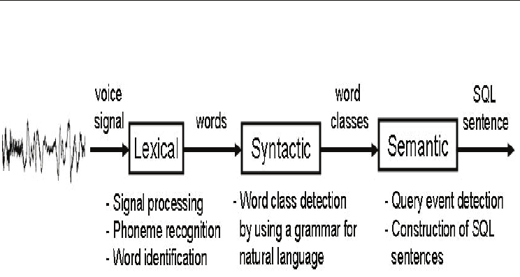
Fig. 1. Flow of data through the three processing components involved in the translation of
queries in spoken natural language to SQL queries.
Our approach to the translation of query phrases from a spoken natural language to SQL is
mainly to detect query events (which are discussed later) by three processing components,
lexical, syntactic and semantic, as depicted in Figure 1, and then translate them as an SQL
expression. The lexical component models common low-layer symbols in both languages to
generate words. The syntactic component exploits the arrangement in the words to
distinguish the associated word classes, e.g., adjective, verb, determiner, subject,
preposition, and adverb, by employing a context-free grammar for natural language. Once
the class of each word is identified, the semantic component checks for valid query events
and builds SQL sentences.
Example 1. Consider the next sentence in Spanish
1
as an example of a query pronounced by
the user.
Recuperar el nombre, el curso y la nota de los alumnos que tengan un profesor
el cual les enseña un curso.
which is translated in English as follows:
Retrieve the name, the course and the grade of the students that have a lecturer
which teach them a course.
We will use this sentence as an aid in presenting the proposed approach in this chapter. !
3.1 Lexical Component
The lexical component of our approach represents the lowest level of abstraction of the
input voice signal captured via a microphone. While the words pronounced by the user are
the basic units of information in spoken natural language, SQL employs a set of keywords
and user-defined literals to express a query expression. Our goal here is to recognize words
expressed in the input voice signal. To this end, we apply a typical signal processing
technique that involves splitting the input signal into small segments by considering
significant pauses in the signal as delimiter, digitizing each signal segment into discrete
values, applying a machine learning algorithm to the discrete values to detect phonemes

Modeling Query Events in Spoken Natural Language for Human-Database Interaction 247
from them, and recognizing valid dictionary words. We believe that the detection of silent
periods in the voice signal and subsequently phonemes, such as /r/, /e/, /c/, /u/, /p/,
/e/, /r/, /a/, and /r/ in recuperar (retrieve in English) leads us to the recognition of the
words pronounced by the user. Since phonemes have a short duration, we analyze each
signal segment by using short-time slicing windows of time length w with the goal of
finding phonemes inside. The window length |w| is an external parameter and should be
long enough to contain phonemes. In the literature this value is commonly set to a value
between 15 to 25 milliseconds [12, 13], and set to 20 milliseconds in our approach. Since
some phonemes may not be detected if they appear in the two consecutive time windows
w1 and w2, we let the third time window w3 overlap w1 and w2 half way in order to capture
the eventual presence of those phonemes. From each window slice, we extract the most
representative features as a vector for further processing. This procedure, denoted as
segmentation in the literature [14], is repeated for the entire voice signal as it arrives through
the microphone.
Among the number of descriptors to extract features from a voice signal within a fixed
length time window, such as Linear Predictive Coding [15], Perceptual Linear Predictive
[16] and RASTA [17], Mel-Frequency Cepstrum Coefficients (MFCC) are widely used
because they have shown to be a robust and accurate approximation method [18]. In
practice, a feature vector of 12MFCC coefficients is enough to characterize any voice
segment. In other words, the entire spoken query can be divided into segments and each
segment is characterized by a feature vector of 12 coefficients. Clustering of these vectors
helps us identify the phonemes contained in the input signal. Among the several existing
clustering methods, we chose the Kohonen’s Self-Organizing Map (SOM) which is trained
with a set of feature vectors, each of which is labeled with a phoneme. The detection of
phonemes in the user speech is then reduced to obtain the neuron with the most similar
feature vector on the SOM. The shape and members of the clusters on the SOM map changes
over time while the SOM learns different phonemes through successive iterations. After
training the SOM, we perform a calibration step where a set of feature vectors with well-
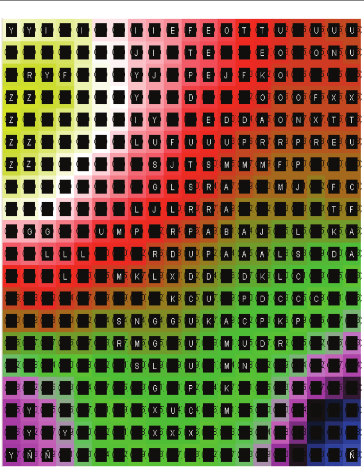
distinguished labels are compared against the map. An example of the resulting map after
training and calibration is depicted in Figure 2. (The signal processing details and program
parameters used in our lexical procedure are fully explained in [19].)
Example 2. Consider the input spoken query in Example 1 again. The SOM training after
calibration recognizes phonemes from the corresponding voice signal. Examples of the
detected phonemes include: /r/, /e/, /c/, /u/, /p/, /e/, /r/, /a/, and /r/ for “recuperar”
(retrieve), /l/, /a/ for “la” (the) and /n/, /o/, /m/, /b/, /r/, and /e/ for “nombre” (name).
Once phonemes are recognized from each signal segment, the detection of words becomes
our final task at this layer. It seems reasonable to think that a sequence of phonemes forms a
word, but some words may not be correctly formed since the presence of noise in the feature
extraction process may lead to the recognition of false positive or false negative phonemes.
Since we are interested in obtaining dictionaryvalid words only, we approximate each word,
formed by a sequence of phonemes, to the most similar word in a dictionary by using the
edit distance as similarity function.
3.2 Syntactic Component
We have obtained a sequence of valid words from the previous lexical component. In the
syntactic component, we employ a lightweight grammar to discover the syntactical
248 Human-Computer Interaction, New Developments
Fig. 2: Illustration of the SOM after the training and calibration process. Note that some
neurons have learned certain phonemes. For example, the phonemes ‘ñ’, ‘y’ and ‘z’ are
treated differently from others in Spanish due to their unique pronounciation. These
phonemes are located, individually or together, in clusters isolated from other phonemes.

Modeling Query Events in Spoken Natural Language for Human-Database Interaction 249
class of each word such as noun, verb, determiner, and adjective from the given word
sequence.
There are different types of grammars that define a language such as context-free, context-
sensitive, deterministic, and non-deterministic. Although all natural languages can be easily
represented by context-sensitive grammars which enable simpler production rules than
other types of grammar, the problem of detecting if a language is generated by a context-
sensitive grammar is PSPACE-complete [20], making it impractical to program such a
language. In contrast to context-sensitive grammars, context-free and deterministic
grammars (Type-2 in the Chomsky hierarchy) are feasible in programming without
generating ambiguous languages and can be recognized in linear time by a finite state
machine. Thus, we propose a context-free, deterministic grammar to process the word
sequence. The proposed grammar is shown in Figure 3 by means of the Backus-Naur Form
notation. The production rules in the grammar identify the syntactical class of each word.
Example 3. By applying the proposed grammar to the words found in the user query
sentence, we obtain the class of each word as follows: recuperar (retrieve:verb), el
(the:determiner), nombre (name:noun), el (the:determiner), curso (course:noun), y (and:copulative-
conjunction), la (the:article), nota (grade:noun), de (of:preposition), los (the:determiner), estudiantes
(students:noun), que (that:preposition), tienen (have:verb), un (a:determiner), profesor
(lecturer:noun), el (the:determiner), cual (which:preposition), les (them:determiner), enseña
(teach:verb), un (a:determiner), curso (course:noun). !
3.3 Semantic Component
In our work, user queries given in the voice stream data are recognized as especial query
events from the sequence of (word:class) pairs generated by the syntactic component. For
this purpose, we propose an event model as follows:
Definition 1 (user query event) A user query is an event that consists of five event
attributes
<What, Where, Who, When, Why>
such that
1. What denotes the target action specified in the given query such as to retrieve, insert,
delete, or update information,
2. Where denotes the set of data sources implied in the query,
3. Who denotes the set of attributes that are presented in the query,
4. When denotes the temporal aspect of the query (optional), and
5. Why denotes a description of the query (optional). !
The role of the what, where and who event attributes are self-explanatory in the definition.
The distance between user queries with respect to time, i.e., the when event attribute, seems
irrelevant in our context since we are focusing on detecting a single

250 Human-Computer Interaction, New Developments
Fig. 3. The grammar used to detect the role of each word
query event from a voice input. Note also that the why event attribute should be defined
ideally as an unambiguous description of the user query to be useful. One way is through
adopting a canonical definition of an event as many authors have considered canonical
MESSAGE −$ verb DIRECTOBJECT
DIRECTOBJECT −$ determiner DETERMINER1
DETERMINER1 −$ determiner DETERMINER2
DETERMINER1 −$ adverb ADVERB1
DETERMINER1 −$ adjective ADJECTIVE1
DETERMINER1 −$ noun NAME1
DETERMINER2 −$ noun NAME1
ADVERB1 −$ adjective ADJECTIVE1
ADJECTIVE1 −$ noun NAME1
ADJECTIVE1 −$ preposition INDIRECTOBJECT
NAME1 −$ . END
NAME1 −$ adjective ADJECTIVE1
NAME1 −$ adverb ADVERB1
NAME1 −$ and ENDLISTOFNAMES
NAME1 −$ adjective ADJECTIVE1
NAME1 −$ preposition INDIRECTOBJECT
NAME1 −$ comparative COMPARATIVE1
NAME1 −$ relative-pronoun CONJUNCTION1
NAME1 −$ copulative-conjunction CONJUNCTION2
NAME1 −$ relative-conjunction NAME2
NAME1 −$ determiner DETERMINER1
ENDLISTOFNAMES −$ determiner determiner1
COMPARATIVE1 −$ to NAME1
COMPARATIVE1 −$ than NAME1
CONJUNCTION2 −$ verb DIRECTOBJECT
CONJUNCTION2 −$ relative-conjunction NAME2
CONJUNCTION2 −$ relative-pronoun CONJUNCTION1
INDIRECTOBJECT −$ the THE1
INDIRECTOBJECT −$ noun NAME1
THE1 −$ table TABLE
TABLE −$ noun NAME1
NAME2 −$ noun CONJUNCTION1
CONJUNCTION1 −$ bool BOOL1
CONJUNCTION1 −$ auxiliary-verb AUXILIARYVERB
CONJUNCTI
ON1 −$ verb VERB1
BOOL1 −$ verb VERB1
AUXILIARYVERB −$ verb VERB1
VERB1 −$ determiner DETERMINER1
VERB1 −$ adjective ADJECTIVE1
VERB1 −$ noun NAME1