Andrews Dawid G. An Introduction to Atmospheric Physics
Подождите немного. Документ загружается.

139 Boundary layers
downward flow into the top of the boundary layer. Using equations (5.47) and (5.49) this
vertical flow can be written in terms of the surface stress component:
w
D
=−
1
ρ
0
f
0
∂τ
(x)
0
∂y
−
∂τ
(y)
0
∂x
. (5.50)
The velocity w
D
is called the Ekman pumping or suction velocity and equation (5.50)
shows that it is proportional to the ‘curl’ of the surface stress.
5.6.2 The laminar Ekman layer
The theory so far has given information only on the vertically integrated properties of the
boundary layer. To look at the vertical structure it is necessary to make an assumption about
the relationship between the frictional stress τ and the velocity. A simple relationship of
this kind is to assume that the stress components are proportional to the vertical gradients
of the horizontal velocity:
τ
(x)
= ρ
0
ν
∂u
∂z
, τ
(y)
= ρ
0
ν
∂v
∂z
. (5.51)
This is clearly analogous to the molecular viscous stress law (4.13). The quantity ν is
the kinematic eddy viscosity and corresponds to the viscosity coefficient η, defined in
equation (4.13), divided by the density. As noted above, we must use the eddy-viscosity
concept with caution.
Using equations (5.51) we now find the vertical structure of the flow within the boundary
layer, again assuming that the flow is steady. In principle the viscosity ν could vary with z,
but we take it to be constant for simplicity. We take f
0
> 0, corresponding to the Northern
Hemisphere.
Under these conditions the pressure-driven flow (u
p
, v
p
) is again geostrophic; since the
boundary layer is shallow, we take (u
p
, v
p
) to be independent of z within the boundary
layer and equal to the large-scale flow (also assumed geostrophic) just above the boundary
layer. For simplicity, we take this large-scale flow to be purely zonal, but varying with the
northward distance y; thus
u
p
= U(y), v
p
= 0, (5.52)
say. (The calculation can be re-worked with v
p
= 0; see Problem 5.8.) The boundary
conditions on the total flow are
(u, v) → (0, 0) as z → 0,
since, with friction, there can be no flow at the ground, and
(u, v) → (U,0) for z D,
assuming that the flow tends to the geostrophic, pressure-driven, value far above the
boundary layer. In terms of the stress-driven flow, these become
(u
τ
, v
τ
) → (−U,0) as z → 0, (5.53)
140 Further atmospheric fluid dynamics
(u
τ
, v
τ
) → (0, 0) for z D, (5.54)
using equations (5.43).Fromequations (5.45), assuming steady flow and using the stress
law (5.51), the stress-driven flow satisfies the coupled differential equations
− f
0
v
τ
= ν
d
2
u
τ
dz
2
, f
0
u
τ
= ν
d
2
v
τ
dz
2
. (5.55)
These can be reduced to a single fourth-order differential equation for u
τ
or v
τ
, but are
more easily solved by introducing the complex quantity
λ
τ
≡ u
τ
+ iv
τ
,
which, from equations (5.55), satisfies the second-order equation
d
2
λ
τ
dz
2
=
if
0
ν
λ
τ
.
The two solutions of this are
λ
τ
∝ exp
±
if
0
ν
1/2
z
= exp
±
(1 + i)
f
0
2ν
1/2
z
. (5.56)
To satisfy the boundary condition (5.54) we must choose the minus sign in equation (5.56),
to ensure exponential decay with z. Then, taking the real and imaginary parts of λ
τ
, applying
the boundary condition (5.53) and adding the pressure-driven flow (5.52),wegetthefull
solution
u = U(y)[1 − e
−z/h
cos(z/h)], (5.57a)
v = U (y)e
−z/h
sin(z/h), (5.57b)
where
h ≡
2ν
f
0
1/2
.
This is Ekman’s solution and the corresponding boundary layer is called the Ekman layer.
We can calculate the corresponding Ekman pumping velocity (5.50) using the stress
law (5.51) and equations (5.57):
w
D
=
ν
2f
0
1/2
−
dU
dy
=
1
2
hξ, (5.58)
where ξ =−dU/dy is the relative vorticity of the free-atmosphere flow. This relation-
ship between w
D
and ξ also holds when the free-atmosphere flow is not purely zonal.
Equation (5.58) shows, for example, that the Ekman pumping velocity is upwards under
a cyclone in the free atmosphere (for which ξ>0) and downwards under an anticyclone
(for which ξ<0).
Figure 5.9 gives a graphical representation (a hodograph) of the horizontal velocity
vector (u, v) as a function of z/h. This diagram is called the Ekman spiral; note how the
velocity vector spirals in towards the free-atmosphere flow (U,0). It is conventional to
define the ‘depth’ of the Ekman layer to be the height at which the horizontal flow first
becomes parallel to the free-atmosphere flow; this corresponds to z = πh = π(2ν/f
0
)
1/2
.
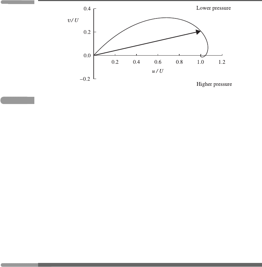
141 Instability
Fig. 5.9
The Ekman spiral: a hodograph of horizontal wind components (normalised by U)intheEkman
layer. The horizontal axis gives the direction of the geostrophic wind above the boundary layer, so
the pressure decreases along the vertical axis. The diagonal arrow indicates the wind vector at a
height z = hπ/2.
Putting this equal to 1 km, the approximate depth of the atmospheric boundary layer, allows
us to get an order-of-magnitude estimate of the value of the eddy viscosity as ν ∼ 5m
2
s
−1
.
(This should be contrasted with the kinematic molecular viscosity of air at STP, which is a
factor of about 10
−5
smaller.)
The Ekman spiral also shows that the deflection of the wind in the boundary layer is
mostly to the low-pressure side of the geostrophic, large-scale flow. Recall from Section 4.8
that the geostrophic flow blows along the isobars; the Ekman-layer analysis indicates how
this is altered in the presence of friction. However, it should be noted that the assump-
tions that have been made in this calculation are seldom fully satisfied in the atmosphere,
owing to the presence of temporal variations and, probably, to the inappropriateness of the
eddy-viscosity concept. As a result, a pure Ekman spiral is hardly ever observed in the real
atmospheric boundary layer.
5.7 Instability
In Section 2.5 we noted that a compressible atmosphere is statically stable if the squared
buoyancy frequency N
2
is positive and statically unstable if it is negative. A similar
criterion, but involving N
2
B
rather than N
2
, applies to an incompressible atmosphere under
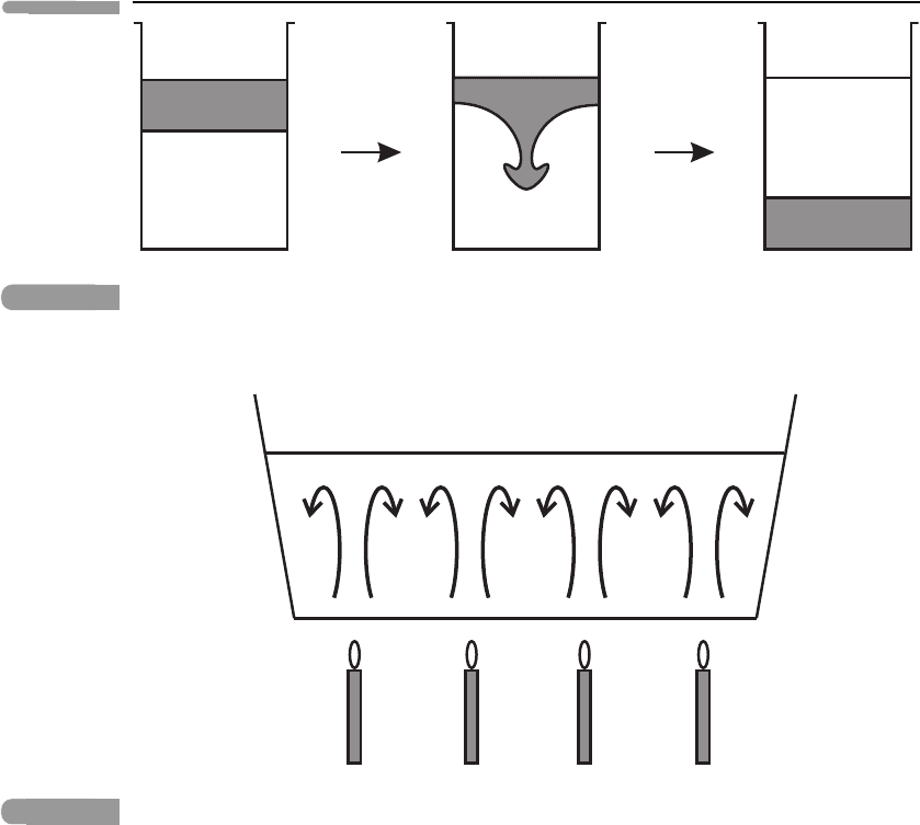
the Boussinesq approximation. Static instability is probably the simplest type of fluid
instability to appreciate: at the most basic level it occurs if a layer of dense, incompressible
fluid of density ρ
2
is introduced over a layer of lighter incompressible fluid of density
ρ
1
<ρ
2
in a closed container (Figure 5.10). In this case the dense fluid will fall through the
lighter fluid, perhaps in a complicated way, leading eventually to a statically stable state in
which the dense fluid is entirely below the light fluid.
A more complex example would be a statically unstable region of finite depth in
a compressible atmosphere. Here parcels displaced adiabatically upwards are ‘lighter’
142 Further atmospheric fluid dynamics
Fig. 5.10
A schematic illustration of static instability in an incompressible fluid. In the left-hand panel,
dense fluid (shaded) is introduced over light fluid (unshaded). Static instability leads to a
redistribution of the fluids; in the final stable state, shown in the right-hand panel, the dense fluid
is entirely below the light fluid.
Fig. 5.11
A schematic illustration of convection patterns in a fluid heated from below and cooled from
above.
(i.e. have a higher potential temperature θ ) than their surroundings and continue to rise,
whereas parcels displaced downwards are ‘heavier’ (i.e. have a lower θ) than their surround-
ings and continue to fall. Eventually a statically stable state is reached, in which low values
of θ are at the bottom and higher values are at the top, so that N
2
= (g/θ)(dθ/dz)>0.
A third case is one in which local regions of static instability are set up by heating from
below, leading to convective instability:seeFigure 5.11 for a laboratory analogue. In the
presence of heating of this kind in the atmosphere we may expect much of the forced region
to approach neutral stability, with N
2
approaching zero and the lapse rate approaching the
dry adiabatic value
a
(see Section 2.5) or the saturated adiabatic value
s
(see Section 2.8)
according to whether the air is unsaturated or saturated.
On large scales, the rotation of the Earth allows more subtle types of instability, which
can lead to important atmospheric disturbances such as cyclones and anticyclones and
other weather phenomena. We briefly discuss the two most important of these: baroclinic
instability and barotropic instability.
143 Instability
5.7.1 Baroclinic instability
Consider a steady zonal flow (U(z),0,0) in the Northern Hemisphere that increases with
height and work with the Boussinesq equations on an f -plane. From geostrophic bal-
ance (5.18) and hydrostatic balance (5.20) we can derive a thermal windshear equation (cf.
equation (4.28b))
f
0
dU
dz
=
g
ρ
0
∂ρ
∂y
,
where ρ =¯ρ(z) + ρ
.SincedU/dz > 0andf
0
> 0 this implies that ∂ρ/∂y > 0, i.e. the
density increases with northward distance. Now the slope α of the density surfaces in the
y, z plane satisfies
tan α ≡
∂z
∂y
ρ
=−
∂ρ/∂y
∂ρ/∂z
by the reciprocity theorem of partial differentiation, equation (4.30). Assuming that the
flow is statically stable, so that ∂ρ/∂z < 0, it follows that tan α>0. Thus a zonal wind
that increases with height is associated, through thermal windshear balance, with density
surfaces that slope polewards and upwards.
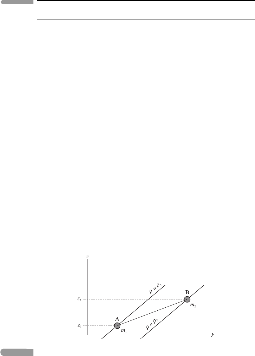
We now show that this configuration of density surfaces may be able to release potential
energy. Suppose that air parcels, each of volume V , are somehow interchanged between
two density surfaces ρ = ρ
1
and ρ = ρ
2
,whereρ
2
>ρ
1
, as shown in Figure 5.12.That
is, parcel A, of mass m
1
= ρ
1
V and at initial height z
1
, is swapped with parcel B, of mass
m
2
= ρ
2
V and initial height z
2
, without any other part of the fluid being disturbed. The
initial potential energy of the two parcels alone is g(m
1
z
1
+m
2
z
2
) while their final potential
energy is g(m
2
z
1
+ m
1
z
2
). There is therefore an increase of potential energy of the two
parcels (and hence of the whole fluid, since no other changes take place) given by
E
P
= g(m
2
z
1
+ m
1
z
2
) − g(m
1
z
1
+ m
2
z
2
)
=−g(m
2
− m
1
)(z
2
− z
1
) =−gV (ρ
2
− ρ
1
)(z
2
− z
1
).
Fig. 5.12 Hypothetical interchange of two parcels from surfaces of different densities.
144 Further atmospheric fluid dynamics
However, ρ
2
>ρ
1
,so,ifz
2
> z
1
,asinFigure 5.12 (that is, the heavier parcel is initially
higher than the lighter parcel), then E
P
< 0; there is thus a decrease of potential energy as
a result of the interchange. This can occur, despite the stable density stratification, because
the density surfaces are sloping more steeply than the line joining the two parcels. There is
then a possibility that the potential energy released by the interchange may be converted to
kinetic energy, leading to unstable motions. These motions are an example of baroclinic
instability, also known as sloping convection.
6
Of course this kind of interchange of
parcels is highly idealised, so further analysis is needed to determine whether it is ever
dynamically possible.
A simple model, which is more realistic and also dynamically consistent, is Eady’s model
of baroclinic instability, in which the background flow is taken to be a linear function of
height, U = Λz, between rigid horizontal boundaries at z = D and z =−D on an f -plane,
with N
B
constant. The corresponding background streamfunction is Ψ =−Λyz and the
background density is a linear function of y.
Linearised quasi-geostrophic disturbances to this flow are considered, and for simplicity
we shall assume that these disturbances are independent of y: they therefore satisfy a
linearised QGPV equation of the form
∂
∂t
+ U
∂
∂x
∂
2
ψ
∂x
2
+
f
2
0
N
2
B
∂
2
ψ
∂z
2
= 0, (5.59)
(cf. equations (5.25) and (5.35)). The boundary conditions are that the vertical velocity
w
a
= 0atz =−D and D; from equation (5.24) this implies that D
g
(∂ψ/∂z) = 0atthe
boundaries. On linearisation about the background flow this gives
∂
∂t
+ U
∂
∂x
∂ψ
∂z
− Λ
∂ψ
∂x
= 0atz =±D. (5.60)
Normal mode solutions of equations (5.59) and (5.60) of the form
ψ
= Re
ˆ
ψ(z) exp[ik(x − ct)] (5.61)
are now sought, where k > 0 and the phase speed c may be complex: c = c
r
+ ic
i
.Itis
found that c
i
> 0 for a certain range of wavenumbers, corresponding to a normal mode that
grows in time like exp(kc
i
t): this exponential growth is a signal of instability. The quantity
kc
i
is called the growth rate; it is the inverse of the e-folding time for the instability. A
brief sketch of the details is as follows.
Substitution of (5.61) into (5.59) gives
ik(U − c)
−k
2
ˆ
ψ +
f
2
0
N
2
B
ˆ
ψ
= 0
6
The word baroclinic in this context refers to the height variation of the zonal wind or the corresponding
latitudinal variation of the density or temperature.
145 Instability
and hence, if U(z) = c,
ˆ
ψ
− K
2
ˆ
ψ = 0, where K =
N
B
k
f
0
;
note that this corresponds to a perturbation QGPV that is zero everywhere. The solutions
can be written
ˆ
ψ = A cosh(Kz) + B sinh(Kz), (5.62)
where A and B are complex constants. Substitution of (5.61) into the boundary
conditions (5.60) gives
z −
c
Λ
ˆ
ψ
−
ˆ
ψ = 0atz =±D.
When expression (5.62) is substituted into each of these boundary conditions, the resulting
equations added and subtracted and then A and B eliminated, we obtain the dispersion
relation
c
2
=−
Λ
2
K
2
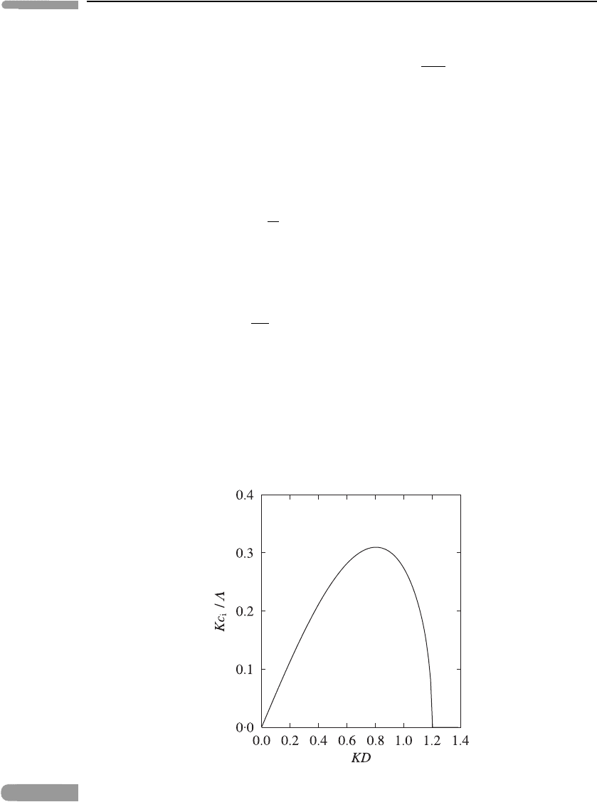
[coth(KD) − KD][KD − tanh(KD)]. (5.63)
It can be shown that the right-hand side of equation (5.63) is negative for 0 < KD 1.2 and
positive otherwise. Therefore we get growing modes (c
i
> 0) for non-zero wavenumbers
k less than about 1.2f
0
/(N
B
D), i.e. horizontal wavelengths greater than about 5.2N
B
D/f
0
;
these unstable modes have c
r
= 0 and do not propagate. The maximum growth rate
kc
i
is about 0.31Λf
0
/N
B
and occurs where k ≈ 0.8f
0
/(N
B
D):seeFigure 5.13. For k
1.2f
0
/(N
B
D), c is real and no growth occurs; the resulting stable modes propagate with
equal and opposite real phase speeds c
r
.
Fig. 5.13
Normalised growth rate Kc
i
/Λ as a function of KD for unstable normal modes in Eady’s model of
baroclinic instability. Note that the ordinate is proportional to the growth rate kc
i
and the abscissa
is proportional to the horizontal wavenumber k.
146 Further atmospheric fluid dynamics
Although the Eady model is highly simplified, it can be generalised in various ways. The
unstable modes that result bear some resemblance to developing cyclones and anticyclones
in the midlatitude troposphere and also to certain unstable waves observed in laboratory
analogues of the atmosphere (see Section 9.4).
5.7.2 Barotropic instability
A different type of instability can occur for basic winds U(y) that vary with the northward
distance y but not with height z; this kind of flow structure is called barotropic.Takingthe
disturbance streamfunction ψ
to be independent of z and retaining the β-effect, we get
∂
∂t
+ U
∂
∂x
∂
2
ψ
∂x
2
+
∂
2
ψ
∂y
2
+
β − U
∂ψ
∂x
= 0,
from linearising the QGPV equation (5.25). We seek normal mode solutions of the f orm
ψ = Re
ˆ
φ(y) exp[ik(x − ct)], (5.64)
where again k > 0andc may be complex, and obtain the second-order ordinary differential
equation
U − c
ˆ
φ
− k
2
ˆ
φ
+
β − U
ˆ
φ = 0. (5.65)
This must be solved subject to suitable boundary conditions; convenient (though not
physically very realistic) ones are that the northward velocity should vanish on east–west
oriented boundaries at y = 0, L, say. Hence
ˆ
φ = 0aty = 0, L. (5.66)
Equations (5.65) and (5.66) form a system with complex eigenvalues c
(n)
= c
(n)
r
+ ic
(n)
i
,
n = 1, 2, 3, ... and corresponding complex eigenfunctions
ˆ
φ
(n)
(y). Unlike the Eady-
problem case, these equations cannot generally be solved analytically; however, they are
straightforward to solve by numerical methods.
The physical interpretation of these solutions is as follows. Suppose that the zonal flow
U(y) is initially undisturbed, for t < 0. At time t = 0 it is given a small perturbation
ψ
0
; this perturbation can be Fourier-analysed into components of differing wavenumber k;
moreover each of these components can in turn be resolved into a linear combination of
the eigenfunctions for that value of k. Each term (or mode) in this sum then evolves in time
according to equation (5.64), with its own complex phase speed. Modes for which c
i
≤ 0
are stable: their amplitudes do not grow with time. However, any modes for which c
i
> 0
will grow exponentially in time like exp(kc
i
t); these are called unstable modes and the
mode with the largest c
i
will eventually outgrow the others and dominate the disturbance.
Thus if unstable modes exist, most initial disturbances will generally excite them and the
flow will rapidly be distorted. (Of course, the exponential growth in this case means that
the assumption of a small disturbance amplitude will eventually break down for sufficiently
large t, whereupon the model ceases to be valid.)

147 Problems
This barotropic instability mechanism is believed to be responsible for a number of
types of large-scale weather disturbance observed in the tropical troposphere, as well
as eddies in the stratosphere. On the other hand, if there are no unstable modes, initial
disturbances will not grow and the flow is not affected very much by the perturbation
imposed at t = 0.
A useful general result is the Rayleigh–Kuo criterion, which states that if β −U
does
not change sign in the region 0 ≤ y ≤ L then all modes are stable. It does not guarantee
that unstable modes will always occur if β − U
vanishes somewhere; however, the latter
condition must hold if there is to be any chance of finding unstable modes.
Further reading
The physical interpretation of vorticity given here follows the approach of Acheson (1990).
Vector-calculus identities like equation (5.3) are given in many mathematics texts, such
as those by Riley et al. (2006)andBoas (1983). The advanced texts on geophysical fluid
dynamics by Vallis (2006), Pedlosky (1987)andGill (1982) cover most of the topics in this
chapter in much more detail than attempted here, and should be consulted by readers who
wish to pursue the subject further. The original derivation of equation (5.40) was given in
the pioneering paper by Charney and Drazin (1961).
Problems
Problem 5.1 Show that the two-dimensional circular flow u = V (r)i
ϕ
introduced in
Section 5.1 can be written in plane Cartesian coordinates (x, y, z) as
u =
V
(x
2
+ y
2
)
1/2
(−y, x,0);
hence or otherwise verify that the z component of the vorticity is
ξ =
dV
dr
+
V
r
,
and that the other components are zero.
Problem 5.2 Pure inertial oscillations (see also Problem 4.3) can be modelled by neglect-
ing horizontal pressure gradients in the linearised Boussinesq equations (5.16a) and (5.16b)
on an f -plane:
u
t
− f
0
v = 0, v
t
+ f
0
u = 0.
Define ˜u = u + iv and solve for (u, v), given that (u, v) = (u
0
,0) at t = 0. Given that
particle displacements (X , Y ) satisfy
∂X
∂t
= u,
∂Y
∂t
= v,
148 Further atmospheric fluid dynamics
show that the particle trajectories for these oscillations are circular. Calculate the radius of
the circle if the particle speed is (a) 1 m s
−1
and (b) 10 m s
−1
.
Problem 5.3 Calculate the horizontal and vertical air-parcel displacements X and Z
associated with an internal gravity wave, defined by X
t
= u and Z
t
= W (cf. Problem 5.2),
given that these displacements vanish when x = z = t = 0. Show that the air parcels
oscillate in straight lines perpendicular to the vector (k,0,m).
Find the period (in minutes) of an internal gravity wave of horizontal wavelength 100 km
and vertical wavelength 5 km in the Earth’s mesosphere, where N
2
B
= 3 × 10
−4
s
−2
.How
long (in minutes) does the information associated with this wave take to propagate through
a vertical distance of 20 km? If the maximum horizontal wind fluctuation (peak-to-peak)
due to the wave is 2 m s
−1
, find the maximum horizontal and vertical distances traversed
by an air parcel.
Problem 5.4 Inertia–gravity waves are the generalisation of the internal gravity waves of
Section 5.4 to the case when f
0
= 0. Look for linear plane-wave solutions of the form (5.27)
and show in particular that
ρ
0
ˆu =
ωk ˆp
ω
2
− f
2
0
, ρ
0
ˆv =
−ikf
0
ˆp
ω
2
− f
2
0
(5.67)
and that the dispersion relation is
ω
2
= f
2
0
+
N
2
B
k
2
m
2
.
Note that the northward velocity v must be non-zero.
What is the minimum angular frequency of these waves? Show that, for a given frequency
and vertical wavelength, these waves have a larger horizontal wavelength than do the
corresponding internal gravity waves.
Problem 5.5 Using equations (5.67) and the hydrostatic equation, calculate the mean
kinetic energy per unit volume
K and the mean available potential energy per unit volume
P, averaged over one wave period. How does the ratio P/K behave when ω → f
0
and when
ω f
0
? To what kind of wave does the latter limit refer? Show that equipartition between
mean kinetic energy and mean available potential energy does not occur for long waves.
Problem 5.6 Starting with the Rossby-wave dispersion relation (5.36), consider waves in
the absence of a background flow, with l = 0. For fixed m put b = f
0
m/N
B
and sketch ω as a
function of k,fork > 0, with particular attention to the limits k → 0andk b. Show that
Rossby waves cannot exist if the wave period is shorter than a critical value. Estimate this
critical period at 45
◦
N for waves of vertical wavelength 10 km, given N
2
B
= 5 ×10
−4
s
−2
,
a value representative of the stratosphere.
Problem 5.7 Consider Rossby waves that vary with x and y but are independent of depth
z, in a uniform zonal flow U. Show that stationary waves can exist only if the zonal (x)